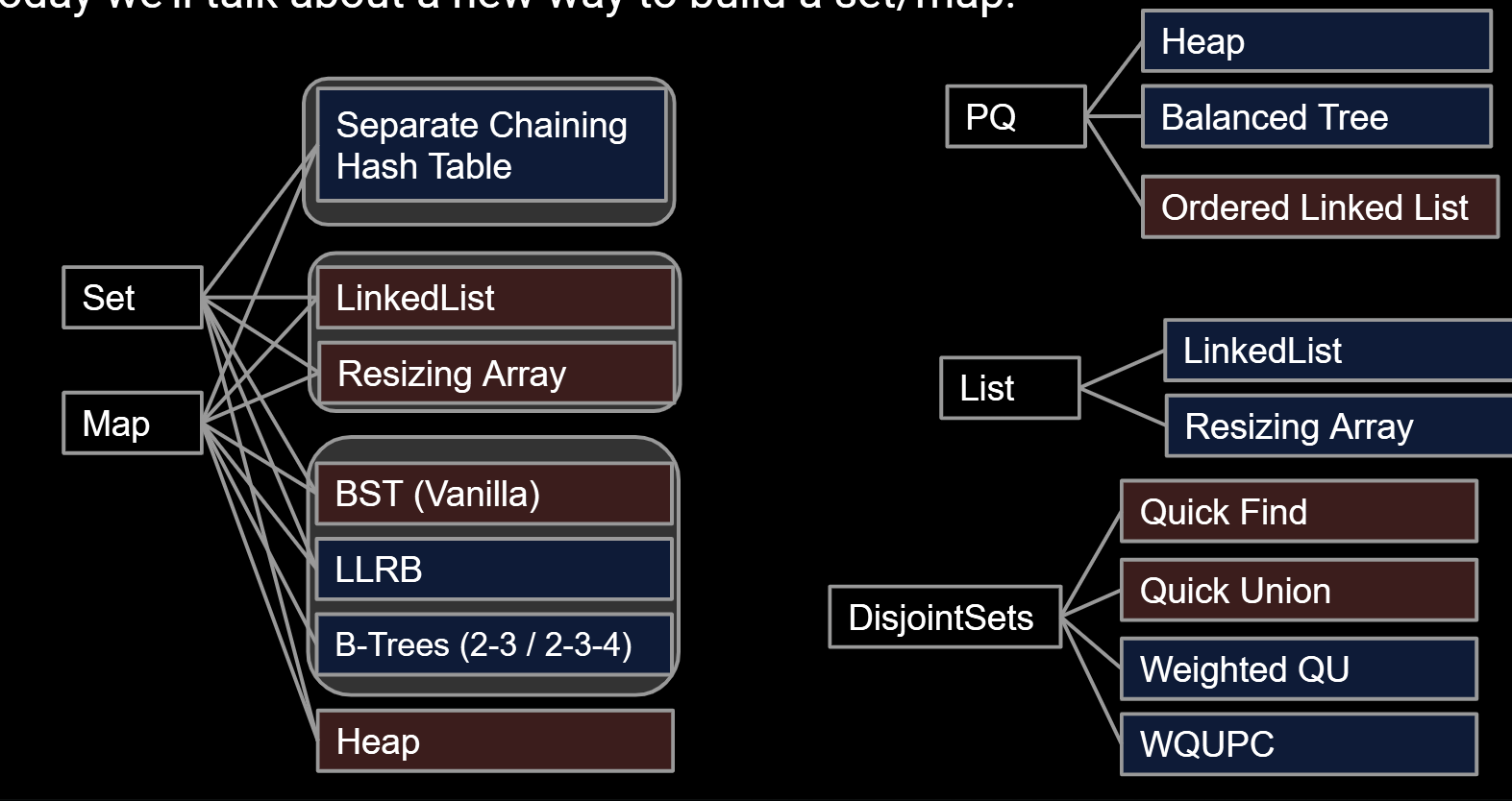
the note of UCB CS61B
|
|
QUOTE
Computer science is essentially about one thing: Managing complexity. ——proj0
redundancy is one our worst enemies when battling complexity! ——proj1
If you are going to be working for something, make sure that what you do actually benefits the world your interpretations——Justin
Syntax knowledge
- Difference between Pass by Value and Pass by Reference
- most of the language’s function is Pass by Value, including C, java, py, meaning they pass the value of parameters into function instead of reference
- note: every data type in C except array is pass by value, for its value is its refrerence
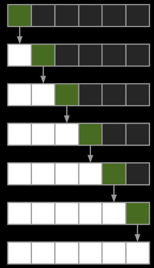
1. Lab 3:Timing Test
1.1 Array Lists(Alists)’s resizing
Alist
|
|
resizing
|
|
However, using [size +1] may cause inefficiency. For example, resizing a alist from 100 to 1000 may need nearly 500,000 operations, for it need to create 100 to 1000 boxes respectively.
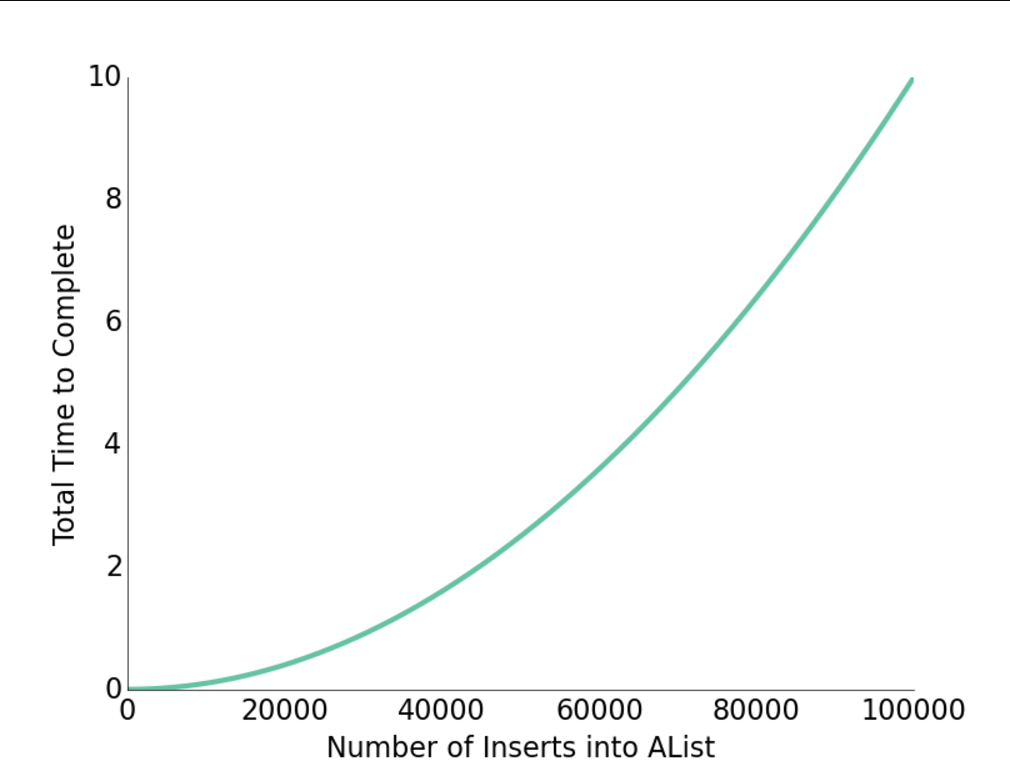
To fix this, using the multiply can lead to surprisingly great performance.
|
|
1.2 loitering
-
Java only destroys unwanted objects when the last reference has been lost.
-
Keeping references to unneeded objects is sometimes called loitering.
Save memory. Don’t loiter.
1.3Obscurantism in Java
We talk of “layers of abstraction” often in computer science.
- Related concept: obscurantism. The user of a class does not and should not know how it works.
- The Java language allows you to enforce this with ideas like private!
- A good programmer obscures details from themselves, even within a class.
- Example: addFirst and resize should be written totally independently. You should not be thinking about the details of one method while writing the other. Simply trust that the other works.
- Breaking programming tasks down into small pieces (especially functions) helps with this greatly!
- Through judicious use of testing, we can build confidence in these small pieces, as we’ll see in the next lecture.
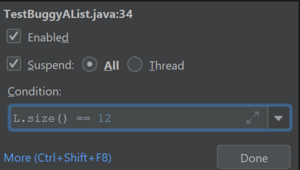
1.4 Conditional Breakpoint & Execution Breakpoint
-
Right-click on your breakpoint and you’ll see a box pop up that says “Condition:”. In the box, type in what condition you want the code to stop.
-
-
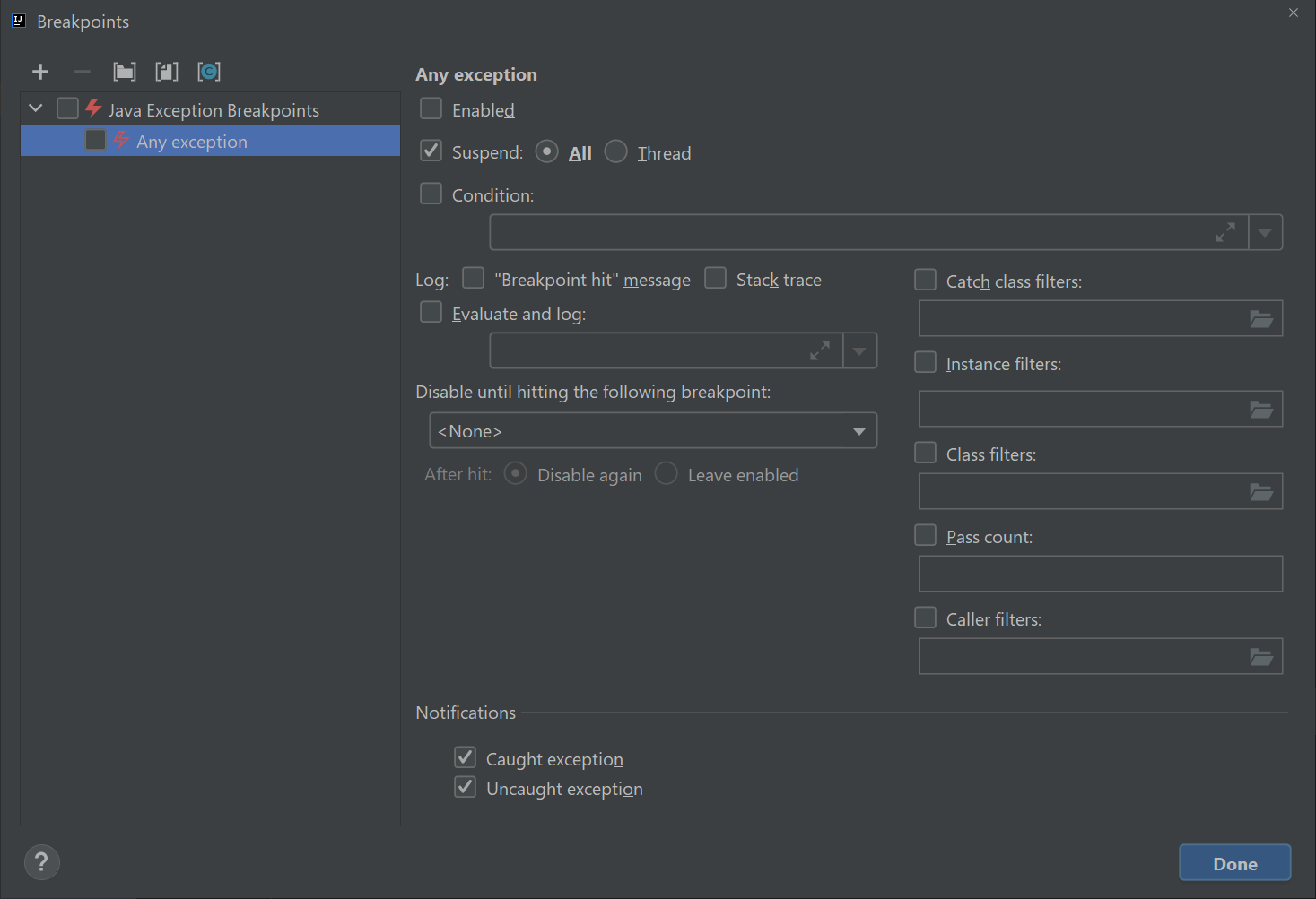
click “Run -> View Breakpoints”. You should see a window like this pop up:
-
Click on the checkbox on the left that says “any exception” and then click on that says “Condition:” and in the window and enter exactly:
1this instanceof java.lang.ArrayIndexOutOfBoundsException -
2.Project 1:Deque
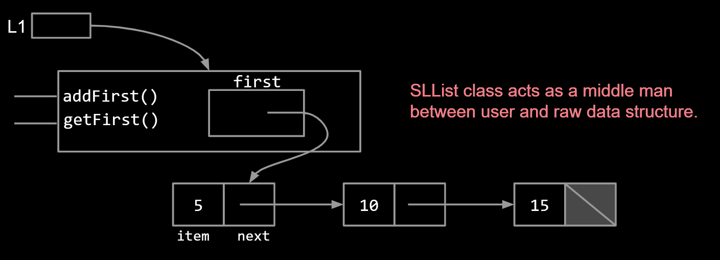
2.1 SLLists
|
|
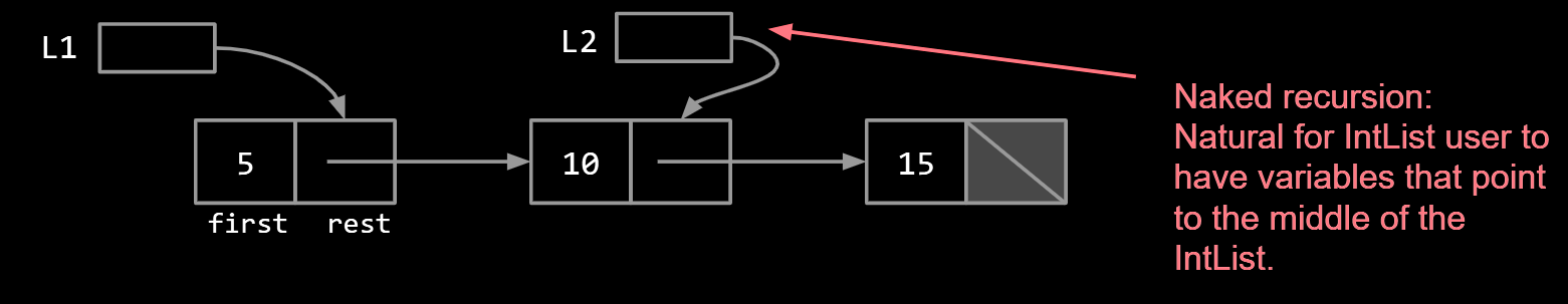
Instead of using a naked recursion which user can gain free access to the variables in the middle of the list, SLList class act as a middle man between user and raw data structure. It’s a kind of encapsulation.
2.2 Sentinel Nodes
Notes:
- I’ve renamed first to be sentinel.
- sentinel is never null, always points to sentinel node.
- Sentinel node’s item needs to be some integer, but doesn’t matter what value we pick.
- Had to fix constructors and methods to be compatible with sentinel nodes.
|
|
2.3 Class variation and Instance variation
The first instance
|
|
The second instance
|
|
| 方面 | 第一种方式 | 第二种方式 |
|---|---|---|
| 数组初始化时机 | 在构造函数中完成 | 在成员变量声明时完成 |
| 灵活性 | 高(可根据构造函数参数动态调整数组大小) | 低(数组大小固定为 8) |
| 代码简洁性 | 较冗长,逻辑分散 | 简洁直观,逻辑集中 |
| 规范性 | 命名不规范,可能混淆 | 更加符合 Java 的常见命名规范 |
| 适用场景 | 需要动态初始化逻辑或多种初始化方案 | 初始化逻辑固定且简单的场景 |
3.Asymptotics(渐进)
Efficiency comes in two flavors:
- Programming cost (course to date. Will also revisit later).
- How long does it take to develop your programs?
- How easy is it to read, modify, and maintain your code?
- More important than you might think!
- Majority of cost is in maintenance, not development!
- Execution cost (from today until end of course).
- How much time does your program take to execute?
- How much memory does your program require?
But, how to compare the efficiency of different algorithm, in a simple and mathematically rigorous.
3.1 Asymptotic Behavior
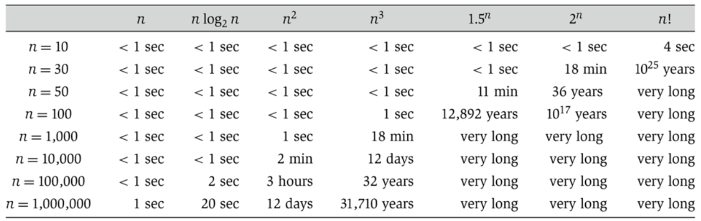
In most cases, we care only about asymptotic behavior, i.e. what happens for very large N.
-
Simulation of billions of interacting particles.
-
Social network with billions of users.
-
Logging of billions of transactions.
-
Encoding of billions of bytes of video data.
3.2 Simplification model
for instance, consider this code which return whether an array contain two same number
|
|
| operation | count |
|---|---|
| i = 0 | 1 |
| j = i + 1 | 1 to $N$ |
| less than (<) | 2 to $(N^2+3N+2)/2$ |
| increment (+=1) | 0 to $(N^2+N)/2$ |
| equals (==) | 1 to $(N^2-N)/2$ |
| array accesses | 2 to $N^2-N$ |
-
Simplification1: consider only the worse case
- Justification: When comparing algorithms, we often care only about the worst case [but we will see exceptions in this course].
-
Simplification 2: Restrict Attention to One Operation
-
Pick some representative operation to act as a proxy for the overall runtime.
in this case, we call our choice the “cost model”
-
Good choice: increment.
-
Bad choice: assignment of j = i + 1.
It might not represent the overall cost as effectively because it could occur too infrequently or might be overshadowed by more significant operations.
-
-
-
Simplification 3: Eliminate low order terms.
-
Simplification 4: Eliminate multiplicative constants.
| operation | worst case o.o.g. |
|---|---|
| increment (+=1) | $N^2$ |
3.3 Big-Theta
| function | order of growth |
|---|---|
| $N^3 + 3N^4$ | $N^4$ |
| $1/N + N^3$ | $N^3$ |
| $1/N + 5$ | 1 |
| $Ne^N + N$ | $Ne^N$ |
| $40 sin(N) + 4N^2$ | $N^2$ |
Suppose we have a function R(N) with order of growth f(N).
- In “Big-Theta” notation we write this as R(N) ∈ Θ(f(N)).
- Examples:
- $N^3 + 3N^4$ ∈ Θ($N^4$)
- $1/N + N^3$ ∈ Θ($N^3$)
- $1/N + 5$ ∈ Θ(1)
- $Ne^N + N$ ∈ Θ($Ne^N$)
- $40 sin(N) + 4N^2$ ∈ Θ($N^2$)
3.4 Big O Notation
$$ R(N) \in O(f(N)) \\ R(N) \leq k_2 \cdot f(N) $$4.Iteration
Java allows us to iterate through Lists and Sets using a convenient shorthand syntax sometimes called the “foreach” or “enhanced for” loop.
|
|
An alternate, uglier way to iterate through a List is to use the iterator() method. Though it is only the shortened version.
|
|
The code on the top is just shorthand for the code below. And the compiler needs to check whether the Set interface have a iterator()
|
|
To support ugly iteration:
- Add an iterator() method to ArraySet that returns an Iterator
. - The Iterator
that we return should have a useful hasNext() and next() method.
|
|
|
|
|
|
|
|
How It Works Together
- The
ArraySetobject (aset) provides an iterator (ArraySetIterator) through theiterator()method. - The
whileloop useshasNext()to check if there are more elements and callsnext()to retrieve each element. - The
ArraySetIteratorinternally keeps track of the position (wizPos) and retrieves elements from theitemsarray.
Lastly, to support the enhanced for loop, we need to make ArraySet implement the Iterable interface.
|
|
So to build a iterator in a real life project
|
|
5.Disjoint Sets
Deriving the “Disjoint Sets” data structure for solving the “Dynamic Connectivity” problem. We will see:
- How a data structure design can evolve from basic to sophisticated.
- How our choice of underlying abstraction can affect asymptotic runtime (using our formal Big-Theta notation) and code complexity.
Goal: Design an efficient Disjoint Sets implementation.
-
Number of elements N can be huge.
-
Number of method calls M can be huge.
-
Calls to methods may be interspersed (e.g. can’t assume it’s onlu connect operations followed by only isConnected operations).
The Disjoint Sets data structure has two operations:
- connect(x, y): Connects x and y.
- isConnected(x, y): Returns true if x and y are connected. Connections can be transitive, i.e. they don’t need to be direct.
5.1.The native approach
Model connectedness in terms of sets.
- How things are connected isn’t something we need to know.
- Only need to keep track of which connected component each item belongs to.
5.1.1 Quick find
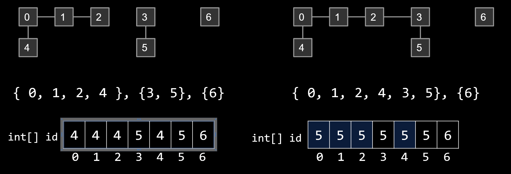
Idea #1: List of sets of integers, e.g. [{0, 1, 2, 4}, {3, 5}, {6}]
- In Java: List<Set
>. - Very intuitive idea.
- Requires iterating through all the sets to find anything. Complicated and slow!
- Worst case: If nothing is connected, then isConnected(5, 6) requires iterating through N-1 sets to find 5, then N sets to find 6. Overall runtime of Θ(N).
| Implementation | constructor | connect | isConnected |
|---|---|---|---|
| ListOfSetsDS | Θ(N) | O(N) | O(N) |
Idea #2: list of integers where ith entry gives set number (a.k.a. “id”) of item i.
- connect(p, q): Change entries that equal id[p] to id[q]
| Implementation | constructor | connect | isConnected |
|---|---|---|---|
| ListOfSetsDS | Θ(N) | O(N) | O(N) |
| QuickFindDS | Θ(N) | Θ(N) | Θ(1) |
5.1.2 Quick Union
Idea: Assign each item a parent (instead of an id). Results in a tree-like shape.
-
An innocuous sounding, seemingly arbitrary solution.
-
Unlocks a pretty amazing universe of math that we won’t discuss.

connect(5, 2)
- One possibility, set id[3] = 2; but you lost the bond between 3 and 5
- Set id[3] = 0; but tree can be to tall to climb
| Implementation | Constructor | connect | isConnected |
|---|---|---|---|
| ListOfSetsDS | Θ(N) | O(N) | O(N) |
| QuickFindDS | Θ(N) | Θ(N) | Θ(1) |
| QuickUnionDS | Θ(N) | O(N) | O(N) |
5.1.3. Weighted Quick Union
Suppose we are trying to connect(2, 5). We have two choices:
- Make 5’s root into a child of 2’s root. Height: 2
- Make 2’s root into a child of 5’s root. Height: 3
Which is the better choice?
Modify quick-union to avoid tall trees.
-
Track tree size (number of elements).
-
New rule: Always link root of smaller tree to larger tree.
Minimal changes needed:
- Use parent[] array as before.
- isConnected(int p, int q) requires no changes.
- connect(int p, int q) needs to somehow keep track of sizes.
- See the Disjoint Sets lab for the full details.
- Two common approaches:
- Use values other than -1 in parent array for root nodes to track size.
- Create a separate size array.
| Implementation | Constructor | connect | isConnected |
|---|---|---|---|
| ListOfSetsDS | Θ(N) | O(N) | O(N) |
| QuickFindDS | Θ(N) | Θ(N) | Θ(1) |
| QuickUnionDS | Θ(N) | O(N) | O(N) |
| WeightedQuickUnionDS | Θ(N) | O(log N) | O(log N) |
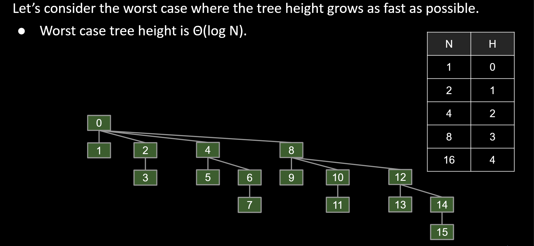
5.1.4 Path Compression: A Clever Idea
Below is the topology of the worst case if we use WeightedQuickUnion
- Clever idea: When we do isConnected(15, 10), tie all nodes seen to the root.
- Additional cost is insignificant (same order of growth).
5.Sets,Maps,Binary Search Trees
Among the most important interfaces in the java.util library are those that extend the Collection interface (btw interfaces can extend other interfaces).
- Lists of things.
- Sets of things.
- Mappings between items, e.g. jhug’s grade is 88.4, or Creature c’s north neighbor is a Plip.
- Maps also known as associative arrays, associative lists (in Lisp), symbol tables, dictionaries (in Python).
5.1Binary Search Trees
To a ordered list, there is a fundamental problem: slow search, though it’s ordered.
So, how to improve it?
5.1.1.BST definition
A tree consists of:
- A set of nodes.
- A set of edges that connect those nodes.
- Constraint: There is exactly one path between any two nodes.
BST Property. For every node X in the tree:
-
Every key in the left subtree is less than X’s key.
-
Every key in the right subtree is greater than X’s key.
- Ordering must be complete, transitive, and antisymmetric. Given keys p and q:
- Exactly one of p ≺ q and q ≺ p are true.
- p ≺ q and q ≺ r imply p ≺ r.
- One consequence of these rules: No duplicate keys allowed!
- Keeps things simple. Most real world implementations follow this rule
- Ordering must be complete, transitive, and antisymmetric. Given keys p and q:
5.1.2 .BST Operations: Search
If searchKey equals T.key, return.
- If searchKey ≺ T.key, search T.left.
- If searchKey ≻ T.key, search T.right.
|
|
The runtime to search a bushy BST is the worse case needs $\Theta(\log N)$ of time, because the height of the tree is ~$\log N$
5.1.3.BST Operations: Insert
when inserting items into BST, search for key.
- If found, do nothing.
- If not found:
- Create new node.
- Set appropriate link.
|
|
Avoid ARMS LENGTH RECURSION, which means break each kind of circumstances into the easiest way, i.e. instead of using T.right.right == nullor T.right == nullor anything like that, use T == null, which is the simplest circumstances.
5.1.4.BST Operations: Delete
Breaking down the circumstances, it has 3 Cases:
- Deletion key has no children.
- Deletion key has one child.
- Deletion key has two children.
#1: with no children
Deletion key has no children (“glut”):
-
Just sever the parent’s link.
-
What happens to “glut” node?
- Garbage collected
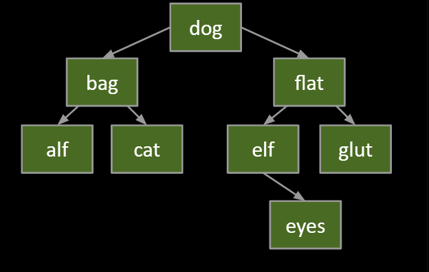
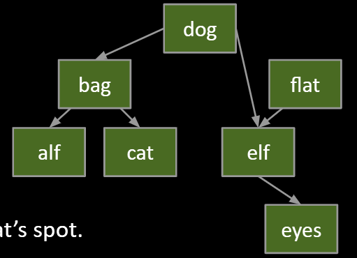
#2: with one children
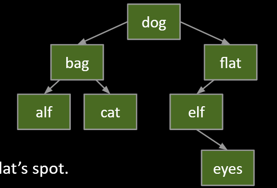
Goal:
- Maintain BST property.
- Flat’s child definitely larger than dog.
- Safe to just move that child into flat’s spot.
Thus: Move flat’s parent’s pointer to flat’s child.
- Flat will be garbage collected (along with its instance variables).
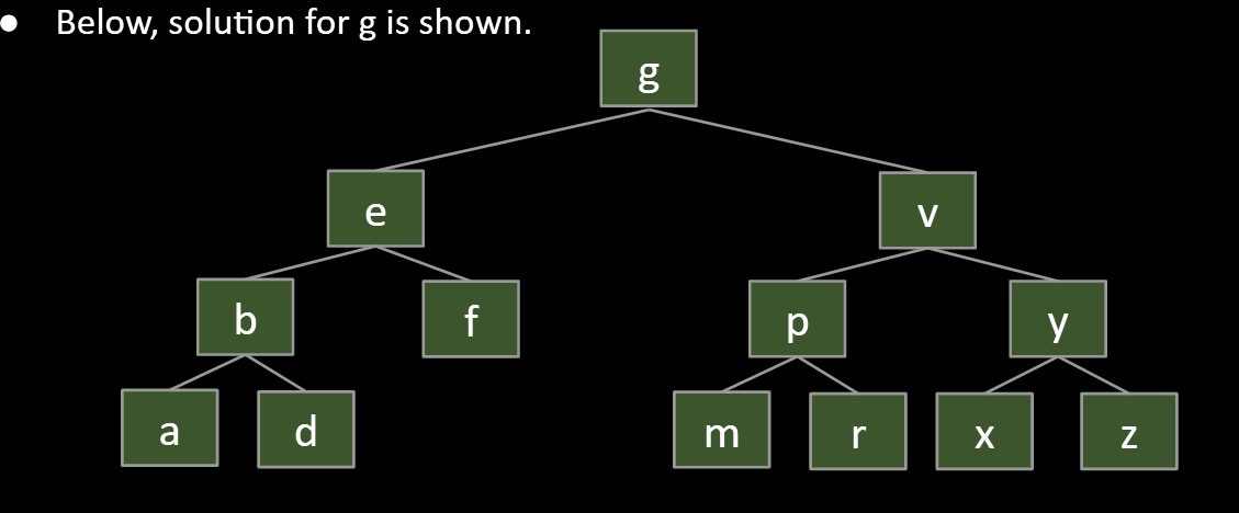
#3: hard challenge
Delete k
Goal:
- Find a new root node.
- Must be > than everything in left subtree.
- Must be < than everything right subtree.
In this case, you can choose predecessor g or successerm to be the new root, why?
They are both larger than the left side and minor than the right side
6.B-Trees
6.1.Intro
BSTs have:
- Worst case Θ(N) height.
- Best case Θ(log N) height.
- Θ(log N) height if constructed via random inserts.
Bad News: We can’t always insert our items in a random order. Why?
- Data comes in over time, don’t have all at once.
- Example: Storing dates of events.
- add(“01-Jan-2019, 10:31:00”)
- add(“01-Jan-2019, 18:51:00”)
- add(“02-Jan-2019, 00:05:00”)
- add(“02-Jan-2019, 23:10:00”)
- Example: Storing dates of events.
6.2.B-trees / 2-3 trees / 2-3-4 trees
Crazy idea: Never add new leaves at the bottom.
- Tree can never get imbalanced.
However: The problem is adding new leaves at the bottom.
Avoid new leaves by “overstuffing” the leaf nodes.
- “Overstuffed tree” always has balanced height, because leaf depths never change.
- Height is just max(depth).
Height is balanced, but we have a new problem:
- Leaf nodes can get too juicy.
Solution?
-
Set a limit L on the number of items, say L=3.
-
If any node has more than L items, give an item to parent.
- Which one? Let’s say (arbitrarily) the left-middle.
- Pulling item out of full node splits it into left and right.
- Parent node now has three children!
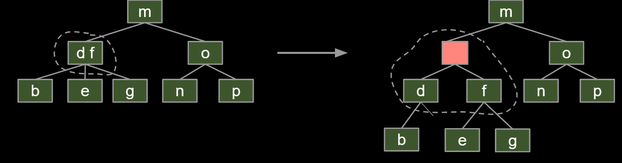
B-tree’s name:
- B-trees of order L=3 (like we used today) are also called a 2-3-4 tree or a 2-4 tree.
- “2-3-4” refers to the number of children that a node can have, e.g. a 2-3-4 tree node may have 2, 3, or 4 children.
- B-trees of order L=2 are also called a 2-3 tree.
B-Trees are most popular in two specific contexts:
- Small L (L=2 or L=3):
- Used as a conceptually simple balanced search tree (as today).
- L is very large (say thousands).
- Used in practice for databases and filesystems (i.e. systems with very large records).
6.3.Runtime analysis
L: Max number of items per node.
Height: Between ~logL+1(N) and ~log2(N)
- Largest possible height is all non-leaf nodes have 1 item.
- Smallest possible height is all nodes have L items.
- Overall height is therefore Θ(log N).
Runtime for contains:
- Worst case number of nodes to inspect: H + 1
- Worst case number of items to inspect per node: L
- Overall runtime: O(HL)
Runtime for add:
- Worst case number of nodes to inspect: H + 1
- Worst case number of items to inspect per node: L
- Worst case number of split operations: H + 1
- Overall runtime: O(HL) = O(L)
7.Red Black Tree
2-3 trees (and 2-3-4 trees) are a real pain to implement, and suffer from performance problems. Issues include:
- Maintaining different node types.
- Interconversion of nodes between 2-nodes and 3-nodes.
- Walking up the tree to split nodes.
7.1.BST Structure and Tree Rotation
7.1.1 Tree Rotation
rotateLeft(G): Let x be the right child of G. Make G the new left child of x.
- Can think of as temporarily merging G and P, then sending G down and left.
- Preserves search tree property. No change to semantics of tree.
7.1.2.Red-Black Trees
Our goal: Build a BST that is structurally identical to a 2-3 tree.
- Since 2-3 trees are balanced, so will our special BSTs.
Possibility 1: Create dummy “glue” nodes.
Result is inelegant. Wasted link. Code will be ugly.
Possibility 2: Create “glue” links with the smaller item off to the left.
Idea is commonly used in practice (e.g. java.util.TreeSet). For convenience, we’ll mark glue links as “red”.
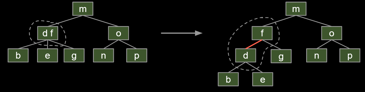
A BST with left glue links that represents a 2-3 tree is often called a “Left Leaning Red Black Binary Search Tree” or LLRB.
- LLRBs are normal BSTs!
- There is a 1-1 correspondence between an LLRB and an equivalent 2-3 tree.
- The red is just a convenient fiction. Red links don’t “do” anything special.
7.2.Maintaining 1-1 Correspondence Through Rotations
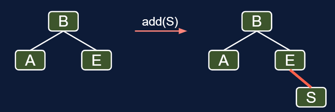
7.2.1. Insertion Color
Use red link when the numbers are on the same leaves
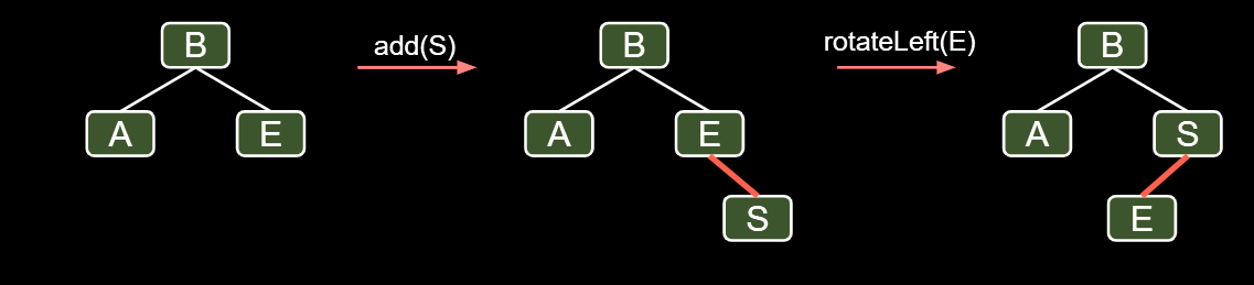
7.2.2.Insertion on the Right
But it’s not leaning left, instead it’s right leaning. So we can use rotateLeft(E)
7.2.3. Double Insertion on the Left
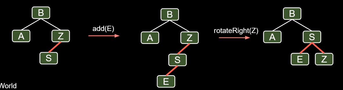
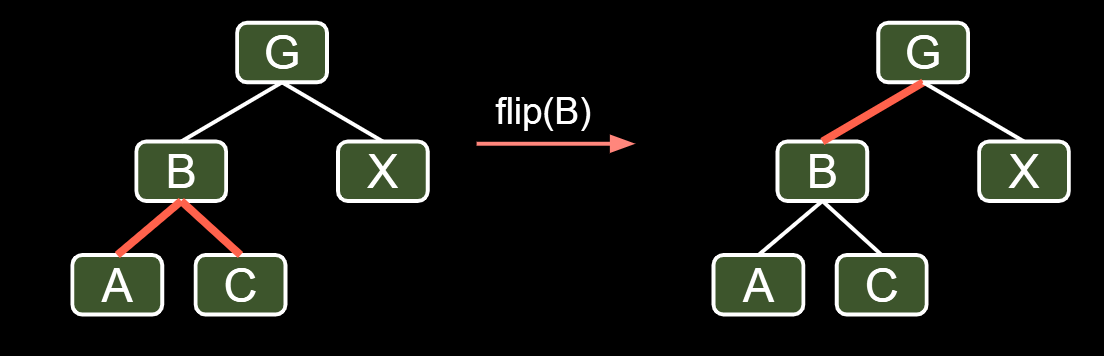
7.2.4.Splitting Temporary 4-Nodes
- Flip the colors of all edges touching B.
- Note: This doesn’t change the BST structure/shape.
7.3.Runtime and Implementation
The runtime analysis for LLRBs is simple if you trust the 2-3 tree runtime.
- LLRB tree has height O(log N).
- Contains is trivially O(log N).
- Insert is O(log N).
- O(log N) to add the new node.
- O(log N) rotation and color flip operations per insert.
|
|
7.4.Search Tree Summary
In the last 3 lectures, we talked about using search trees to implement sets/maps.
- Binary search trees are simple, but they are subject to imbalance.
- 2-3 Trees (B Trees) are balanced, but painful to implement and relatively slow.
- LLRBs insertion is simple to implement (but delete is hard).
- Works by maintaining mathematical bijection with a 2-3 trees.
- Java’s TreeMap is a red-black tree (not left leaning).
- Maintains correspondence with 2-3-4 tree (is not a 1-1 correspondence).
- Allows glue links on either side (see Red-Black Tree).
- More complex implementation, but significantly (?) faster.
8.Hashing
| contains(x) | add(x) | Notes | |
|---|---|---|---|
| ArraySet | Θ(N) | Θ(N) | |
| BST | Θ(N) | Θ(N) | Random trees are Θ(log N). |
| 2-3 Tree | Θ(log N) | Θ(log N) | Beautiful idea. Very hard to implement. |
| LLRB | Θ(log N) | Θ(log N) | Maintains bijection with 2-3 tree. Hard to implement. |
Our search tree based sets require items to be comparable. Not all data type can be asked bigger or smaller. And is it possible to work better than $\Theta)\log N$?
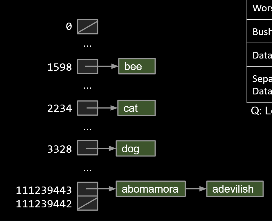
8.1.DataIndexedEnglishWordSet
The core thinking: Using Data as an Index.
You can create a infinite array and use the integer as the array index and put the int into its array.$\Theta (1)$ for add and contain.
Ideally, we want a data indexed set that can store arbitrary types. For instance, turn the boolean box “C” to True if you put “cat” in.
What’s wrong with this approach?
- Other words start with c.
- contains(“chupacabra”) : true
- Can’t store “=98yae98fwyawef”
So, how can we create a unique index for every word?
Use all digits by multiplying each by a power of 27.
- a = 1, b = 2, c = 3, …, z = 26
- Thus the index of “cat” is $(3 \times 27^2) + (1 \times 27^1) + (20 \times 27^0) = 2234.$
As long as we pick a base ≥ 26, this algorithm is guaranteed to give each lowercase English word a unique number!
|
|
8.2.DataIndexedStringSet
Using only lowercase English characters is too restrictive.
- What if we want to store strings like “2pac” or “eGg!”?
- To understand what value we need to use for our base, let’s discuss briefly discuss the ASCII standard.
- Examples:$bee_{126}= (98 \times 126^2) + (101\times 126^1) + (101 \times 126^0) = 1,568,675$
And going beyond the ASCII, you can use UNICODE, allowing Chinese and Japanese too
- $守门员_{40959} = (23432 \times 40959^2) + (38376 \times 40959^1) + (21592 \times 40959^0) = 39,312,024,869,368$
However, this can lead to Integer Overflow and Hash Codes
In Java, the largest possible integer is 2,147,483,647.
- If you go over this limit, you overflow, starting back over at the smallest integer, which is -2,147,483,648.
- In other words, the next number after 2,147,483,647 is -2,147,483,648.
- With base 126, we will run into overflow even for short strings. Pigeonhole principle tells us that if there are more than 4294967296 possible items, multiple items will share the same hash code.
Two fundamental challenges:
-
How do we resolve hashCode collisions (“melt banana” vs. “subterrestrial anticosmetic”)?
- We’ll call this collision handling.
-
How do we compute a hash code for arbitrary objects?
- We’ll call this computing a hashCode.
- Example: Our hashCode for “melt banana” was 839099497.
- For Strings, this was relatively straightforward (treat as a base 27 or base 126 or base 40959 number).
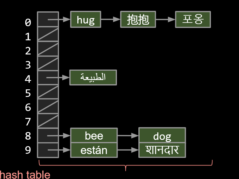
8.3.Hash Tables: Handling Collisions
Suppose N items have the same numerical representation h:
Instead of storing true in position h, store a “bucket” of these N items at position h.
How to implement a “bucket”?
- Conceptually simplest way: LinkedList.
- Could also use ArrayLists.
- Could also use an ArraySet.
- Will see it doesn’t really matter what you do.
Each bucket in our array is initially empty. When an item x gets added at index h:
- If bucket h is empty, we create a new list containing x and store it at index h.
- If bucket h is already a list, we add x to this list if it is not already present.
| Worst case time | contains(x) | add(x) |
|---|---|---|
| Bushy BSTs | Θ(log N) | Θ(log N) |
| DataIndexedArray | Θ(1) | Θ(1) |
| Separate Chaining Data Indexed Array | Θ(Q) | Θ(Q) |
Q: Length of longest list
Observation: We don’t really need billions of buckets. Can use modulus of hashcode to reduce bucket count.
-
Downside: Lists will be longer.
-
What we’ve just created here is called a hash table.
- Data is converted by a hash function into an integer representation called a hash code.
The hash code is then reduced to a valid index, usually using the modulus operator, e.g. 2348762878 % 10 = 8.
Suppose we have:
- An increasing number of buckets M.
- An increasing number of items N.
As long as M = Θ(N), then O(N/M) = O(1).
One example strategy: When N/M is ≥ 1.5, then double M.
- We often call this process of increasing M “resizing”.
- N/M is often called the “load factor”. It represents how full the hash table is.
- This rule ensures that the average list is never more than 1.5 items long!
Assuming items are evenly distributed (as above), lists will be approximately N/M items long, resulting in Θ(N/M) runtimes.
- Our doubling strategy ensures that N/M = O(1).
- Thus, worst case runtime for all operations is Θ(N/M) = Θ(1).
- … unless that operation causes a resize.
| contains(x) | add(x) | |
|---|---|---|
| Bushy BSTs | Θ(log N) | Θ(log N) |
| DataIndexedArray | Θ(1) | Θ(1) |
| Separate Chaining Hash Table With No Resizing | Θ(N) | Θ(N) |
| … With Resizing | Θ(1)† | Θ(1)*† |
*: Indicates “on average”.
†: Assuming items are evenly spread.
8.4.Hash Tables in Java
Hash tables are the most popular implementation for sets and maps.
- Great performance in practice.
- Don’t require items to be comparable.
- Implementations often relatively simple.
- Python dictionaries are just hash tables in disguise.
In Java, implemented as java.util.HashMap and java.util.HashSet.
- How does a HashMap know how to compute each object’s hash code?
- Good news: It’s not “implements Hashable”.
- Instead, all objects in Java must implement a .hashCode() method. Default implementation simply returns the memory address of the object.
Suppose that (glodden apple)‘s hash code is -1.
- Unfortunately, -1 % 4 = -1. Will result in index errors!
- Use Math.floorMod instead.
|
|
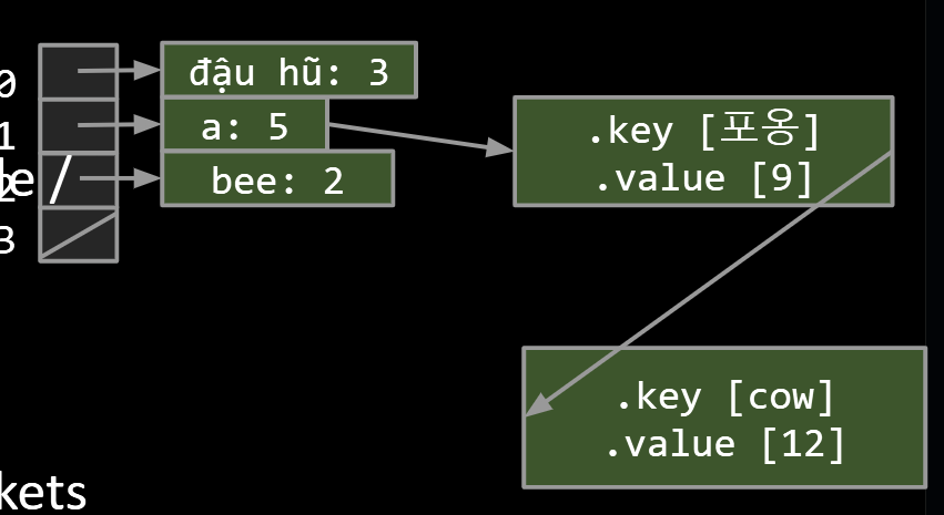
Someone asks me (the hash table) for “cow”:
- Hashcode of cow % array size: get back 1
- !n.key.equals(“cow”) so go to next.
- !n.key.equals(“cow”) so go to next.
- n.key.equals(“cow”), so: return n.value
Warning #1: Never store objects that can change in a HashSet or HashMap!
- If an object’s variables changes, then its hashCode changes. May result in items getting lost.
Warning #2: Never override equals without also overriding hashCode.
- Can also lead to items getting lost and generally weird behavior.
- HashMaps and HashSets use equals to determine if an item exists in a particular bucket.
- See study guide problems.
9.Priority Queues and Heaps
9.1.Priority Queue
Priority Queue Interface
|
|
Useful if you want to keep track of the “smallest”, “largest”, “best” etc. seen so far.
You can have a list with all elements and track the top M elements, but it cost too much memory. Or you could track top M transactions using only M memory.
Some possibilities:
- Ordered Array
- Bushy BST: Maintaining bushiness is annoying. Handling duplicate priorities is awkward.
- HashTable: No good! Items go into random places.
| Ordered Array | Bushy BST | Hash Table | Heap | |
|---|---|---|---|---|
| add | Θ(N) | Θ(log N) | Θ(1) | |
| getSmallest | Θ(1) | Θ(log N) | Θ(N) | |
| removeSmallest | Θ(N) | Θ(log N) | Θ(N) | |
| Caveats | Dups tough |
9.2.Heaps
BSTs would work, but need to be kept bushy and duplicates are awkward.
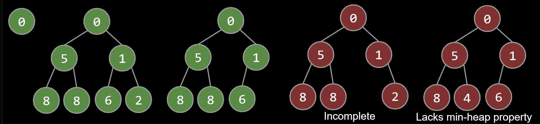
Binary min-heap: Binary tree that is complete and obeys min-heap property.
- Min-heap: Every node is less than or equal to both of its children.
- Complete: Missing items only at the bottom level (if any), all nodes are as far left as possible.
Given a heap, how do we implement PQ operations?
- getSmallest() - return the item in the root node.
- add(x) - place the new employee in the last position, and promote as high as possible.
- removeSmallest() - assassinate the president (of the company), promote the rightmost person in the company to president. Then demote repeatedly, always taking the ‘better’ successor.
See https://goo.gl/wBKdFQ for an animated demo.
9.3.Tree Representations
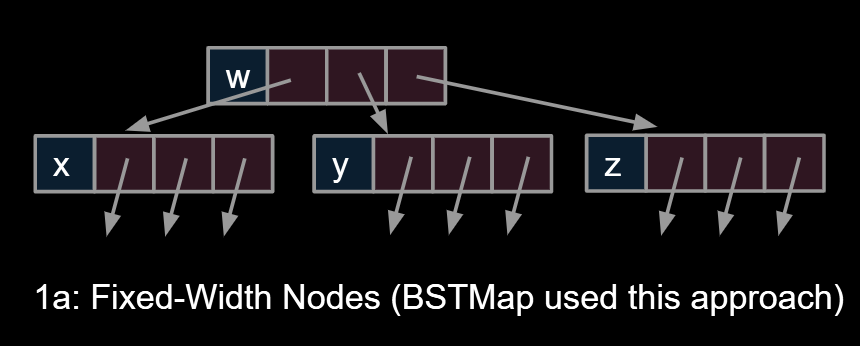
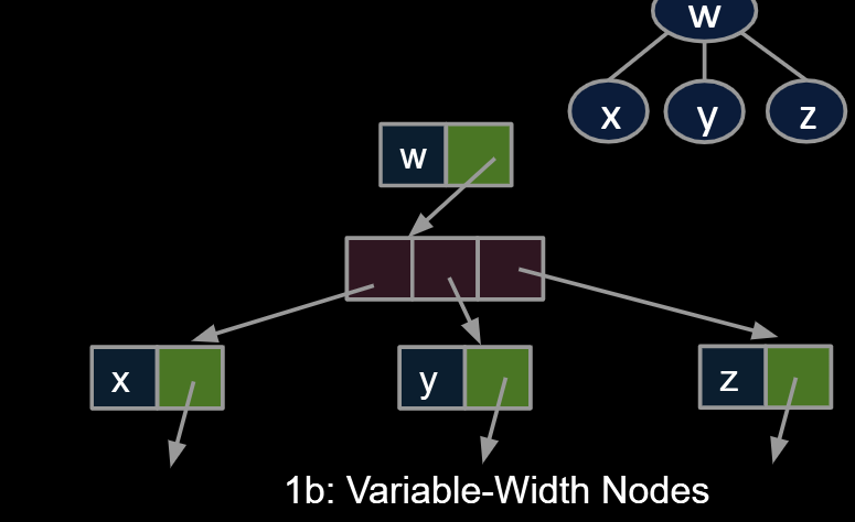
9.3.1.Approach 1
Approach 1a, 1b and 1c: Create mapping from node to children.
1a:Fixed-Width Nodes
|
|
1b:Variable-Width Nodes
|
|
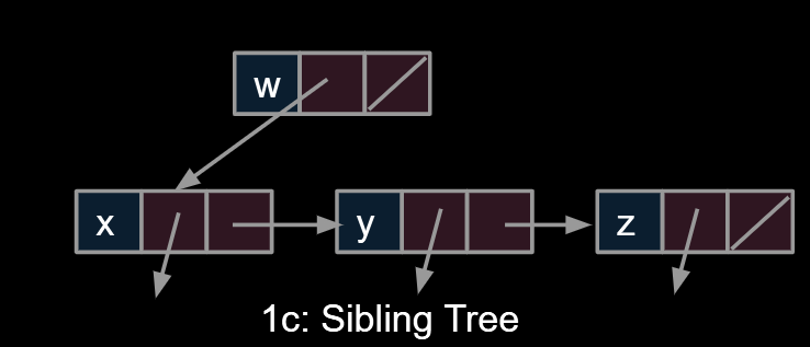
1c:Sibling Tree
|
|
9.3.2.Approach 2
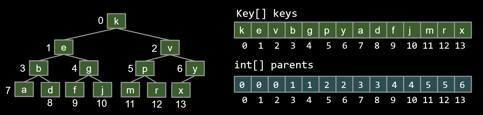
Approach 2: Store keys in an array. Store parentIDs in an array.
- Similar to what we did with disjointSets
|
|
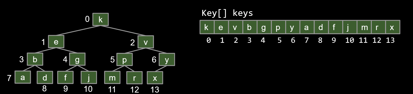
9.3.3.Approach 3
Approach 3: Store keys in an array. Don’t store structure anywhere.
- To interpret array: Simply assume tree is complete.
- Obviously only works for “complete” trees.
|
|
Challenge: Write the parent(k) method for approach 3.
|
|
|
|
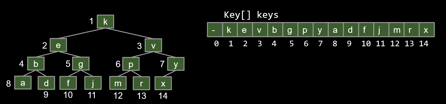
Except there can be a small trick: Store keys in an array. Offset everything by 1 spot.
- Same as 3, but leave spot 0 empty.
- Makes computation of children/parents “nicer”.
- leftChild(k) = k*2
- rightChild(k) = k*2 + 1
- parent(k) = k/2
| Ordered Array | Bushy BST | Hash Table | Heap | |
|---|---|---|---|---|
| add | Θ(N) | Θ(log N) | Θ(1) | Θ(log N) |
| getSmallest | Θ(1) | Θ(log N) | Θ(N) | Θ(1) |
| removeSmallest | Θ(N) | Θ(log N) | Θ(N) | Θ(log N) |
Notes:
- Why “priority queue”? Can think of position in tree as its “priority.”
- Heap is log N time AMORTIZED (some resizes, but no big deal).
- BST can have constant getSmallest if you keep a pointer to smallest.
- Heaps handle duplicate priorities much more naturally than BSTs.
- Array based heaps take less memory (very roughly about 1/3rd the memory of representing a tree with approach 1a).
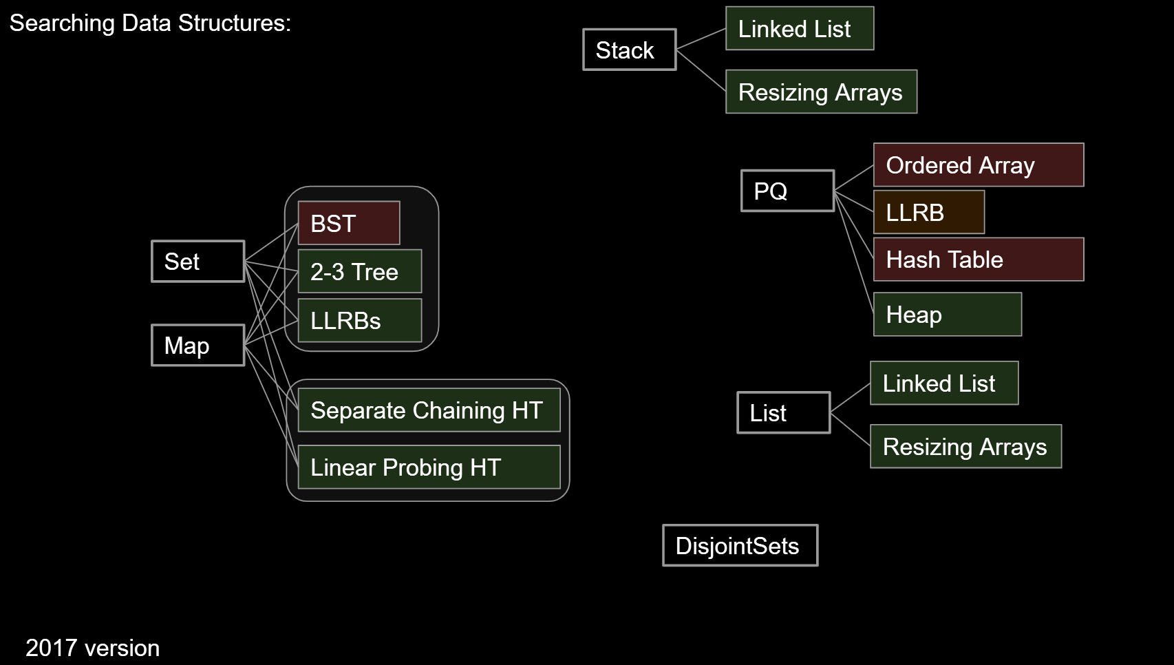
9.4. Data Structure Summary
| Name | Storage Operation(s) | Primary Retrieval Operation | Retrieve By: |
|---|---|---|---|
| List | add(key)insert(key, index) | get(index) | index |
| Map | put(key, value) | get(key) | key identity |
| Set | add(key) | containsKey(key) | key identity |
| PQ | add(key) | getSmallest() | key order (a.k.a. key size) |
| Disjoint Sets | connect(int1, int2) | isConnected(int1, int2) | two int values |

Data Structure: A particular way of organizing data.
- We’ve covered many of the most fundamental abstract data types, their common implementations, and the tradeoffs thereof.
- We’ll do two more in this class:
- Tries, graphs.
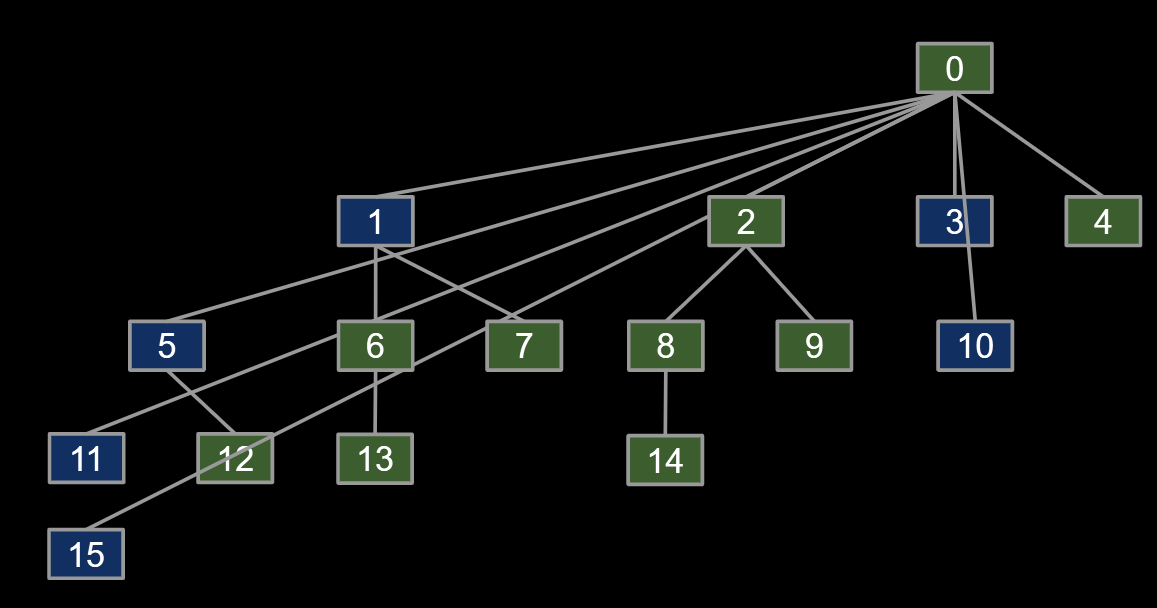
10.Graphs and Traversals
10.1.Trees and Traversals
Trees are a more general concept.
- Organization charts.
- Family lineages* including phylogenetic trees.
- MOH Training Manual for Management of Malaria
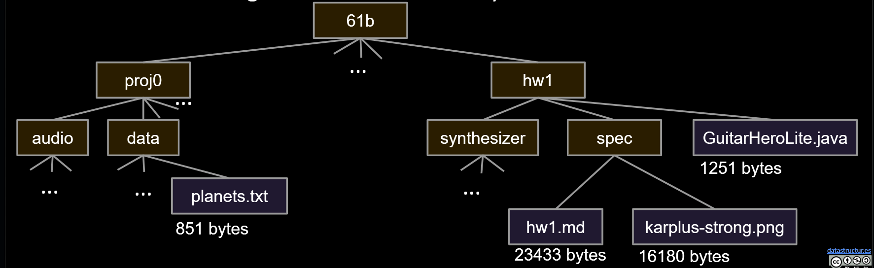
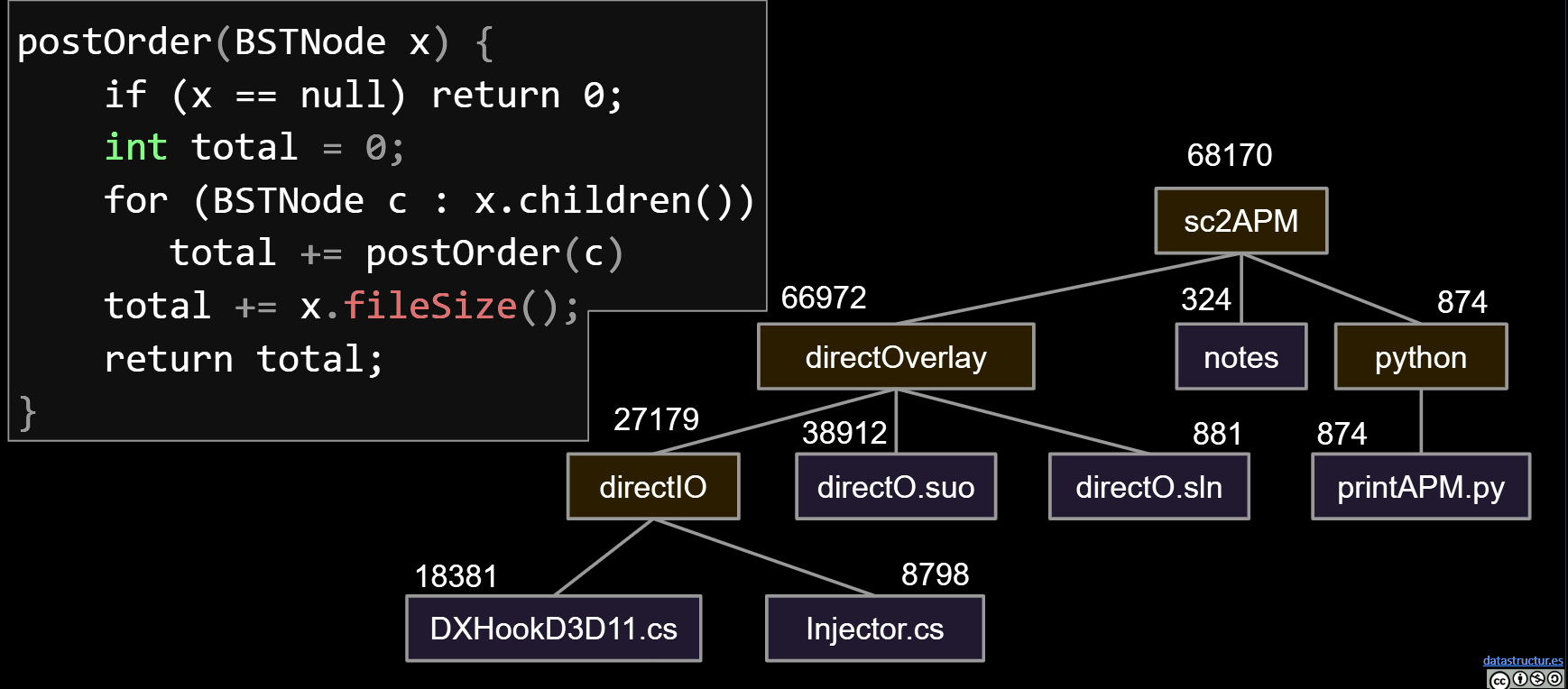
Sometimes you want to iterate over a tree. For example, suppose you want to find the total size of all files in a folder called 61b.
- What one might call “tree iteration” is actually called “tree traversal.”
- Unlike lists, there are many orders in which we might visit the nodes.
- Each ordering is useful in different ways.
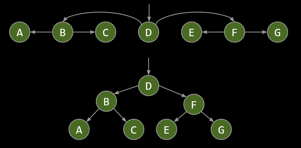
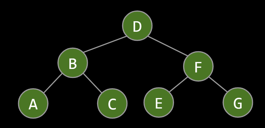
Depth First Traversals
- 3 types: Preorder, Inorder, Postorder
- Basic (rough) idea: Traverse “deep nodes” (e.g. A) before shallow ones (e.g. F).
- Note: Traversing a node is different than “visiting” a node. See next slide.
|
|
|
|
|
|
Example: Tree traversals:
- Preorder: DBACFEG
- Inorder: ABCDEFG
- Postorder: ACBEGFD
- Level order: DBFACEG
Example: Preorder Traversal for printing directory listing:
Example: Postorder Traversal for gathering file sizes.
10.2.Graphs
Trees are fantastic for representing strict hierarchical relationships.
- But not every relationship is hierarchical.
- Example: Paris Metro map.
A graph consists of:
- A set of nodes.
- A set of zero or more edges, each of which connects two nodes. So all trees are graphs!
- The graph can be directed or undirected
A simple graph is a graph with:
- No edges that connect a vertex to itself, i.e. no “loops”.
- No two edges that connect the same vertices, i.e. no “parallel edges”.
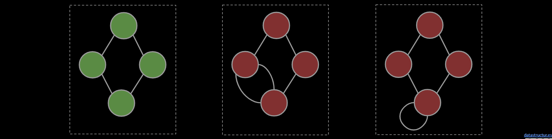
In 61B, unless otherwise explicitly stated, all graphs will be simple.
- In other words, when we say “graph”, we mean “simple graph.”
10.3.Depth-First Traversal
Let’s solve a classic graph problem called the s-t connectivity problem.
- Given source vertex s and a target vertex t, is there a path between s and t?
One possible recursive algorithm for connected(s, t).
- Does s == t? If so, return true.
- Otherwise, if connected(v, t) for any neighbor v of s, return true.
- Return false.
What is wrong with it? Can get caught in an infinite loop. Example:
- connected(0, 7):
- Does 0 == 7? No, so…
- if (connected(1, 7)) return true;
- connected(1, 7):
- Does 1 == 7? No, so…
- If (connected(0, 7)) … ← Infinite loop.
Better version: recursive algorithm for connected(s, t).
- Mark s.
- Does s == t? If so, return true.
- Otherwise, if connected(v, t) for any unmarked neighbor v of s, return true.
- Return false.
This idea of exploring a neighbor’s entire subgraph before moving on to the next neighbor is known as Depth First Traversal.
- Called “depth first” because you go as deep as possible.
- DFS is a very powerful technique that can be used for many types of graph problems.
10.4.Tree Vs. Graph Traversals
Just as there are many tree traversals:
- Preorder, Inorder, Postorder, Level order
So too are there many graph traversals, given some source:
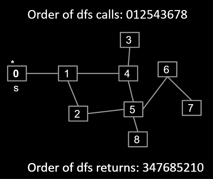
- DFS Preorder: 012543678 (dfs calls).
- DFS Postorder: 347685210 (dfs returns).
- BFS order: Act in order of distance from s.
- BFS stands for “breadth first search”.
- Analogous to “level order”. Search is wide, not deep.
- 0 1 24 53 68 7
11.Graphs II: Graph Traversal Implementations
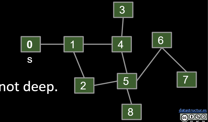
11.1.BFS Answer
Breadth First Search.
- Initialize a queue with a starting vertex s and mark that vertex.
- A queue is a list that has two operations: enqueue (a.k.a. addLast) and dequeue (a.k.a. removeFirst).
- Let’s call this the queue our fringe.
- Repeat until queue is empty:
- Remove vertex v from the front of the queue.
- For each unmarked neighbor n of v:
- Mark n.
- Set edgeTo[n] = v (and/or distTo[n] = distTo[v] + 1).
- Add n to end of queue.
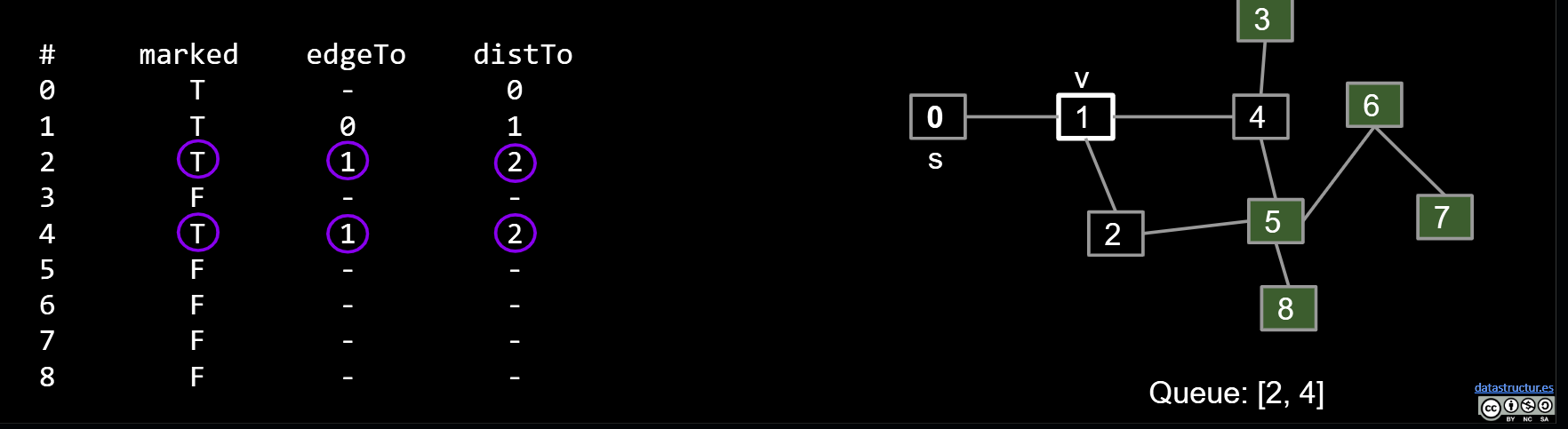
BreadthFirstPaths Implements list
Goal: Find shortest path between s and every other vertex.
- Initialize the fringe (a queue with a starting vertex s) and mark that vertex.
- Repeat until fringe is empty
- Remove vertex v from fringe.
- For each unmarked neighbor n of v: mark n, add n to fringe, set
edgeTo[n] = v, setdistTo[n] = distTo[v] + 1.
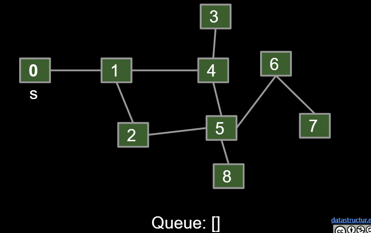
The Queue will turned form [ ]->[0]->[1]->[2,4]->[4,5]->[5,3]->[3,6,8]->[6,8]->[8,7]->[7]->[ ]
11.2.Graph API
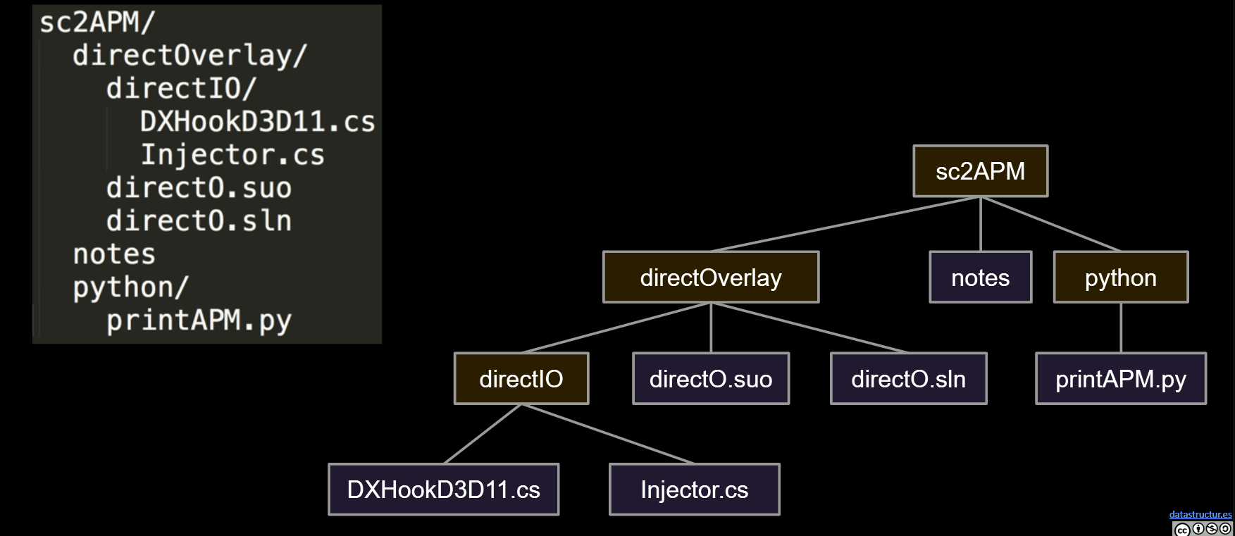
To Implement our graph algorithms like BreadthFirstPaths and DepthFirstPaths, we need:
- An API (Application Programming Interface) for graphs.
- For our purposes today, these are our Graph methods, including their signatures and behaviors.
- Defines how Graph client programmers must think.
- An underlying data structure to represent our graphs.
Our choices can have profound implications on:
- Runtime.
- Memory usage.
- Difficulty of implementing various graph algorithms.
|
|
Print Client:
|
|
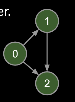
Representation: Adjacency lists.
- Common approach: Maintain array of lists indexed by vertex number.
- Most popular approach for representing graphs.
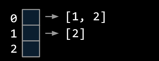
Runtime: Θ(V + E)
- V is total number of vertices
- E is total number of edges in the entire graph
| idea | addEdge(s, t) | for(w : adj(v)) | print() | hasEdge(s, t) | space used |
|---|---|---|---|---|---|
| adjacency matrix | Θ(1) | Θ(V) | Θ(V2) | Θ(1) | Θ(V2) |
| list of edges | Θ(1) | Θ(E) | Θ(E) | Θ(E) | Θ(E) |
| adjacency list | Θ(1) | Θ(1) to Θ(V) | Θ(V+E) | Θ(degree(v)) | Θ(E+V) |
Upper Implementation can be seen in this slide
Bare-Bones Undirected Graph Implementation
|
|
11.3.Graph Traversal Implementations and Runtime
|
|
|
|
|
|
Very hard question: Could we say the runtime is O(E)? No.(E is the number of vertices)
Can’t say O(E)!
- Constructor has to create an all false marked array.
- This marking of all vertices as false takes Θ(V) time.
Our cost model earlier (dfs calls + marked checks) does not provide a tight bound.
| Problem | Problem Description | Solution | Efficiency (adj. list) |
|---|---|---|---|
| s-t paths | Find a path from s to every reachable vertex. | DepthFirstPaths.javaDemo | O(V+E) timeΘ(V) space |
| s-t shortest paths | Find a shortest path from s to every reachable vertex. | BreadthFirstPaths.javaDemo | O(V+E) timeΘ(V) space |
Interesting fact:
- ANY recursive algorithm can be implemented using iteration and a stack.
- In 61C, you’ll learn how recursive calls are implemented at a low level using a stack, i.e. in REAL recursive code, there is an explicit stack being utilized (but below the level of abstraction that you usually think about).
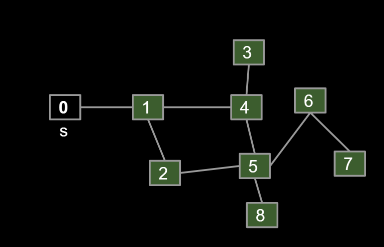
The Stack will go from []->[0]->[1]->[4,2]->[5,3,2]->[8,6,3,2]->[6,3,2]->[7,3,2]->[3,2]->[2]->[]
Visit order [0,1,4,5,8,6,7,3,2]
12.Shortest Path
BFS vs. DFS for Path Finding Possible considerations:
- Correctness. Do both work for all graphs?
- Yes!
- Output Quality. Does one give better results?
- BFS is a 2-for-1 deal, not only do you get paths, but your paths are also guaranteed to be shortest.
- Time Efficiency. Is one more efficient than the other?
- Should be very similar. Both consider all edges twice. Experiments or very careful analysis needed.
- DFS is worse for spindly graphs.
- Call stack gets very deep.
- Computer needs Θ(V) memory to remember recursive calls (see CS61C).
- BFS is worse for absurdly “bushy” graphs.
- Queue gets very large. In worst case, queue will require Θ(V) memory.
- Example: 1,000,000 vertices that are all connected. 999,999 will be enqueued at once.
- Note: In our implementations, we have to spend Θ(V) memory anyway to track distTo and edgeTo arrays.
- Can optimize by storing distTo and edgeTo in a map instead of an array.
BFS yields the wrong route from s to t.
- No: BFS yields a route of length ~190 instead of ~110.
- We need an algorithm that takes into account edge distances, also known as “edge weights”!
12.1.Dijkstra’s Algorithm
Will start with a bad algorithm and then successively improve it.
- Algorithm begins in state below. All vertices unmarked. All distances infinite. No edges in the SPT.
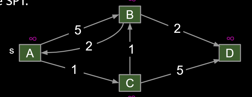
Bad algorithm #1: Perform a depth first search. When you visit v:
- For each edge from v to w, if w is not already part of SPT, add the edge.****
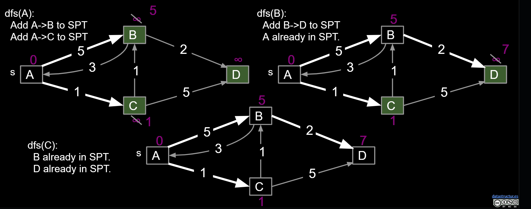
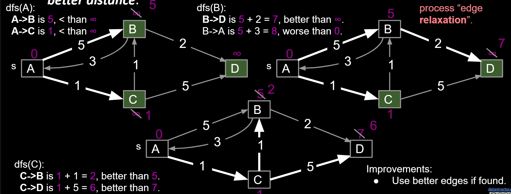
Bad algorithm #2: Perform a depth first search. When you visit v:
- For each edge from v to w, add edge to the SPT only if that edge yields better distance.(We’ll call this process “edge relaxation)
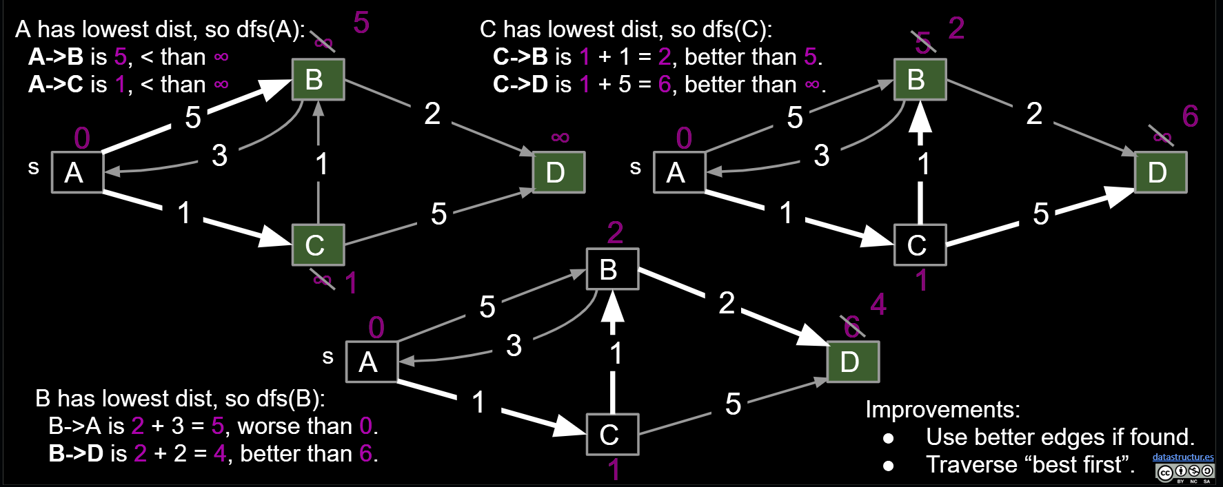
Dijkstra’s Algorithm: Perform a best first search (closest first). When you visit v:
- For each from v to w, relax that edge. i.e. add edge only if that edge yields better distance. See Demo
- Create a priority queue (min-heap) to store vertices, where the priority is the current distance of a vertex.
- Visit vertices in order of best-known distance from source,i.e. the vertices’ distance to source. On visit, relax every edge from the visited vertex. Once visited, the vertex is finalized, its distance can’t be changed. Because before visiting, it is the smallest in the PQ, you can’t expect the further vertex adding a positive number bigger than the finalized value, if all distance is positive.
- So Dijkstra’s is guaranteed to return a correct result if all edges are non-negative. And you don;t need to check if relax is needed if you point at a finalized vertex.
Proof sketch: Assume all edges have non-negative weights.
- At start, distTo[source] = 0, which is optimal.
- After relaxing all edges from source, let vertex v1 be the vertex with minimum weight, i.e. that is closest to the source. Claim: distTo[v1] is optimal, and thus future relaxations will fail. Why?
- distTo[p] ≥ distTo[v1] for all p, therefore
- distTo[p] + w ≥ distTo[v1]
- Can use induction to prove that this holds for all vertices after dequeuing.
12.2.$A^*$
Is this a good algorithm for a navigation application?
- Will it find the shortest path?
- Will it be efficient?
The Problem with Dijkstra’s
- Dijkstra’s will explore every place within nearly two thousand miles of Denver before it locates NYC.
How can we do better?
- Find a way that add up the distance from the vertex to the source and the terminal. It will ideally get a line linking the source and terminal.
- Visit vertices in order of d(Denver, v) + h(v, goal), where h(v, goal) is an estimate of the distance from v to our goal NYC.
- In other words, look at some location v if:
- We know already know the fastest way to reach v.
- AND we suspect that v is also the fastest way to NYC taking into account the time to get to v.
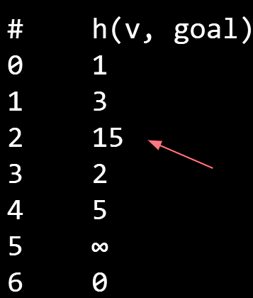
How do we get our estimate?
- Estimate is an arbitrary heuristic h(v, goal).
- heuristic: “using experience to learn and improve”
- Doesn’t have to be perfect!
Single Source, Single Target:
- Dijkstra’s is inefficient (searches useless parts of the graph).
- Can represent shortest path as path (with up to V-1 vertices, but probably far fewer).
- A* is potentially much faster than Dijkstra’s.
- Consistent heuristic guarantees correct solution.
| Problem | Problem Description | Solution | Efficiency |
|---|---|---|---|
| paths | Find a path from s to every reachable vertex. | DepthFirstPaths.javaDemo | O(V+E) timeΘ(V) space |
| shortest paths | Find the shortest path from s to every reachable vertex. | BreadthFirstPaths.javaDemo | O(V+E) timeΘ(V) space |
| shortest weighted paths | Find the shortest path, considering weights, from s to every reachable vertex. | DijkstrasSP.javaDemo | O(E log V) timeΘ(V) space |
| shortest weighted path | Find the shortest path, consider weights, from s to some target vertex | A*: Same as Dijkstra’s but with h(v, goal) added to priority of each vertex.Demo | Time depends on heuristic.Θ(V) space |
13.Minimum Spanning Trees
Given an undirected graph, a spanning tree T is a subgraph of G, where T:
- Is connected.
- Is acyclic(无环).
- Includes all of the vertices.
A minimum spanning tree is a spanning tree of minimum total weight.
- Example: Directly connecting buildings by power lines.
A shortest paths tree depends on the start vertex:
- Because it tells you how to get from a source to EVERYTHING.
There is no source for a MST.
Nonetheless, the MST sometimes happens to be an SPT for a specific vertex.
A Useful Tool for Finding the MST: Cut Property
- A cut is an assignment of a graph’s nodes to two non-empty sets.
- A crossing edge is an edge which connects a node from one set to a node from the other set.
- Cut property: Given any cut, minimum weight crossing edge is in the MST.
Start with no edges in the MST.
- Find a cut that has no crossing edges in the MST.
- Add smallest crossing edge to the MST.
- Repeat until V-1 edges.
- This should work, but we need some way of finding a cut with no crossing edges!
- Random isn’t a very good idea.
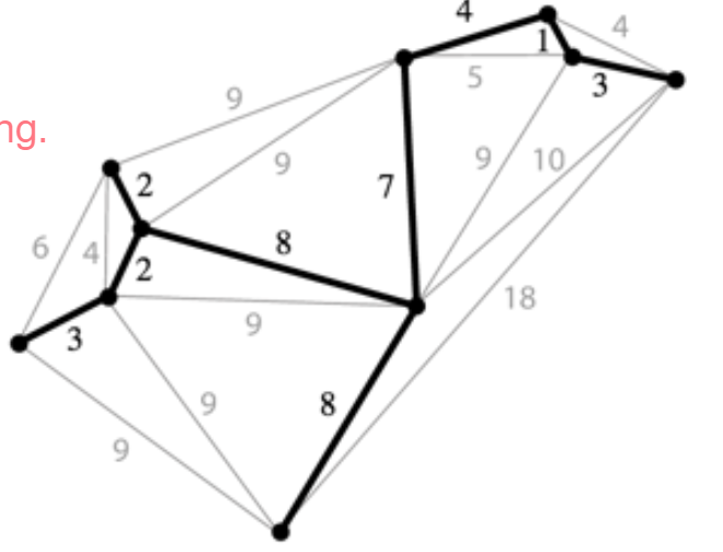
13.1.Prim’s Algorithm
Start from some arbitrary start node.
-
Repeatedly add shortest edge (mark black) that has one node inside the MST under construction.
-
Repeat until V-1 edges.
-
It is very similar with the Dijkstra Algorithm.
-
Visit order:
- Dijkstra’s algorithm visits vertices in order of distance from the source.
- Prim’s algorithm visits vertices in order of distance from the MST under construction.
Relaxation:
-
Relaxation in Dijkstra’s considers an edge better based on distance to source.
-
Relaxation in Prim’s considers an edge better based on distance to tree.
-
-
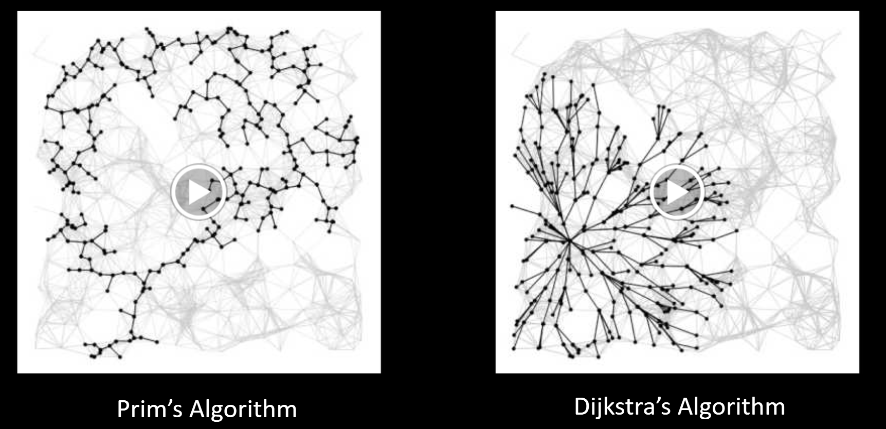
Conceptual Prim’s Algorithm Demo (Link)
Why does Prim’s work? Special case of generic algorithm.
- Suppose we add edge e = v->w.
- Side 1 of cut is all vertices connected to start, side 2 is all the others.
- No crossing edge is black (all connected edges on side 1).
- No crossing edge has lower weight (consider in increasing order).
Prim’s Implementation Pseudocode
|
|
| # Operations | Cost per operation | Total cost | |
|---|---|---|---|
| PQ add | V | O(log V) | O(V log V) |
| PQ delMin | V | O(log V) | O(V log V) |
| PQ decreasePriority | O(E) | O(log V) | O(E log V) |
E stands for number of edges, V stands for number of vertexes. Heap can be one of the PQ.
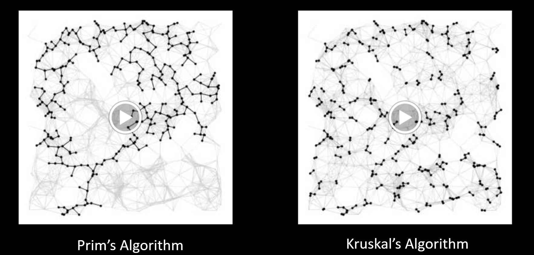
13.2.Kruskal’s Algorithm
Initially mark all edges gray.
- Consider edges in increasing order of weight.
- Add edge to MST (mark black) unless doing so creates a cycle.
- Repeat until V-1 edges.
Conceptual Kruskal’s Algorithm Demo (Link)
Realistic Kruskal’s Algorithm Implementation Demo (Link)
Why does Kruskal’s work? Special case of generic MST algorithm.
- Suppose we add edge e = v->w.
- Side 1 of cut is all vertices connected to v, side 2 is everything else.
- No crossing edge is black (since we don’t allow cycles).
- No crossing edge has lower weight (consider in increasing order).
- It is fundamental a implementation of the Cut property
-
Kruskal’s Implementation (Pseudocode)
|
|
| Operation | Number of Times | Time per Operation | Total Time |
|---|---|---|---|
| Insert | E | O(log E) | O(E log E) |
| Delete minimum | O(E) | O(log E) | O(E log E) |
| union | O(V) | O(log* V) | O(V log* V) |
| isConnected | O(E) | O(log* V) | O(E log*V) |
E stands for number of edges, V stands for number of vertexes.
| Problem | Algorithm | Runtime (if E > V) | Notes |
|---|---|---|---|
| Shortest Paths | Dijkstra’s | O(E log V) | Fails for negative weight edges. |
| MST | Prim’s | O(E log V) | Analogous to Dijkstra’s. |
| MST | Kruskal’s | O(E log E) | Uses WQUPC. |
| MST | Kruskal’s with pre-sorted edges | O(E log* V) | Uses WQUPC. |
14.Directed Acyclic Graphs
Graph problem so far.
| Problem | Problem Description | Solution | Efficiency |
|---|---|---|---|
| paths | Find a path from s to every reachable vertex. | DepthFirstPaths.javaDemo | O(V+E) timeΘ(V) space |
| shortest paths | Find the shortest path from s to every reachable vertex. | BreadthFirstPaths.javaDemo | O(V+E) timeΘ(V) space |
| shortest weighted paths | Find the shortest path, considering weights, from s to every reachable vertex. | DijkstrasSP.javaDemo | O(E log V) timeΘ(V) space |
| shortest weighted path | Find the shortest path, consider weights, from s to some target vertex | A*: Same as Dijkstra’s but with h(v, goal) added to priority of each vertex.Demo | Time depends on heuristic.Θ(V) space |
| minimum spanning tree | Find a minimum spanning tree. | LazyPrimMST.javaDemo | O(???) timeΘ(???) space |
| minimum spanning tree | Find a minimum spanning tree. | PrimMST.javaDemo | O(E log V) timeΘ(V) space |
| minimum spanning tree | Find a minimum spanning tree. | KruskalMST.javaDemo | O(E log E) timeΘ(E) space |
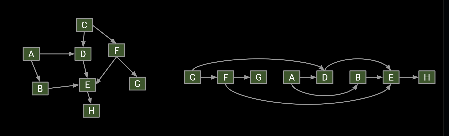
14.1.Topological(拓扑) Sorting
The reason it’s called topological sort: Can think of this process as sorting our nodes so they appear in an order consistent with edges, e.g. [C, F, G, A, D, B, E, H]
- When nodes are sorted in diagram, arrows all point rightwards.
| Problem | Problem Description | Solution | Efficiency |
|---|---|---|---|
| topological sort | Find an ordering of vertices that respects edges of our DAG. | DemoTopological.java | O(V+E) timeΘ(V) space |
DAG: directed acyclic graph
14.2.Shortest Paths on DAGs
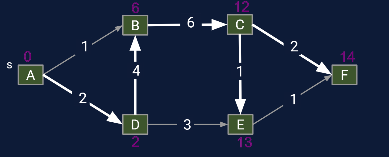
When you want to find the shortest path in a graph, you might use Dijkstra algorithm, but it might fail if we allow negative edges.
- For example, below we see Dijkstra’s just before vertex C is visited.
- Relaxation on E succeeds, but distance to F will never be updated.
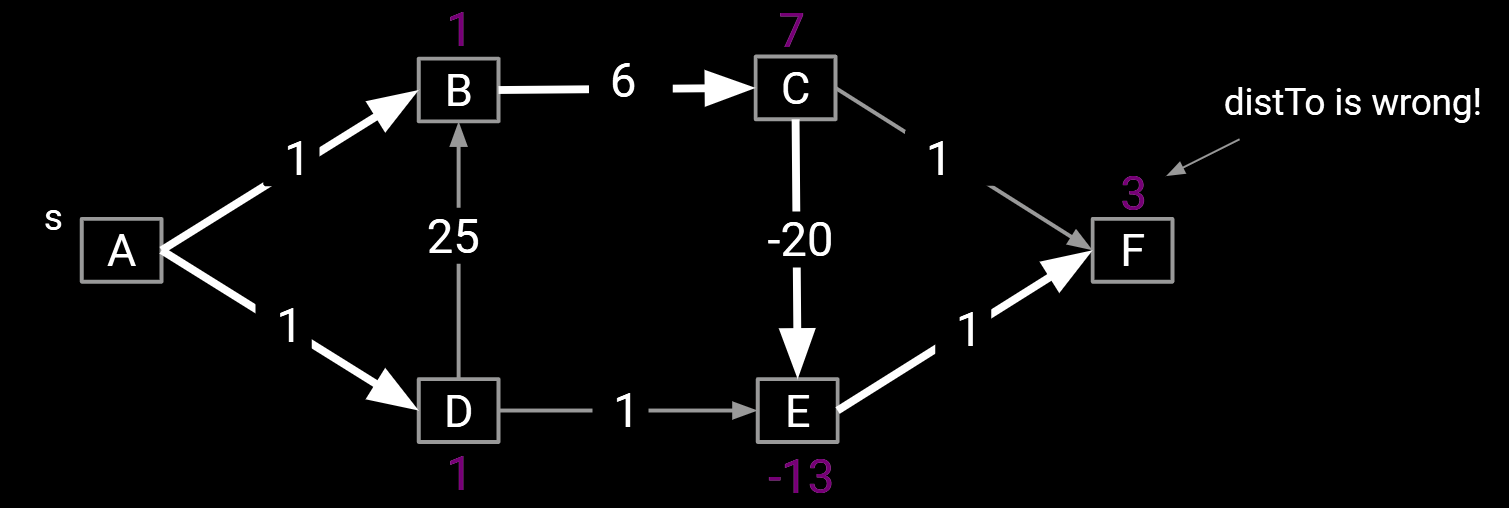
How to imply a feasible algorithm to find the shortest path in a graph with negative edges.
One simple idea: Visit vertices in topological order.
- On each visit, relax all outgoing edges.
- Each vertex is visited only when all possible info about it has been used!
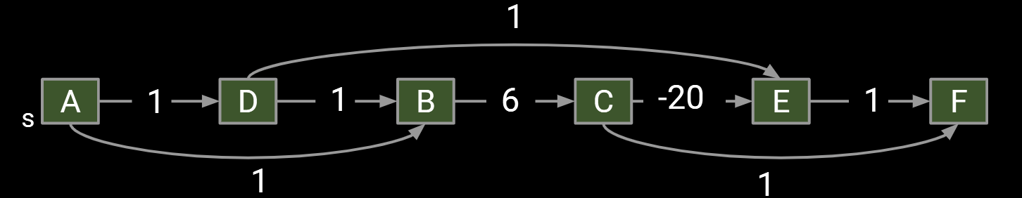
Visit vertices in topological order.(From left to right)
- When we visit a vertex: relax all of its going edges.
- Runtime for step 2 is also O(V + E).
| Problem | Problem Description | Solution | Efficiency |
|---|---|---|---|
| topological sort | Find an ordering of vertices that respects edges of our DAG. | DemoCode: Topological.java | O(V+E) timeΘ(V) space |
| DAG shortest paths | Find a shortest paths tree on a DAG. | DemoCode: AcyclicSP.java | O(V+E) timeΘ(V) space |
14.3.Longest Paths
Consider the problem of finding the longest path tree (LPT) from s to every other vertex. The path must be simple (no cycles!).
Some surprising facts:
- Best known algorithm is exponential (extremely bad).
- Perhaps the most important unsolved problem in mathematics.
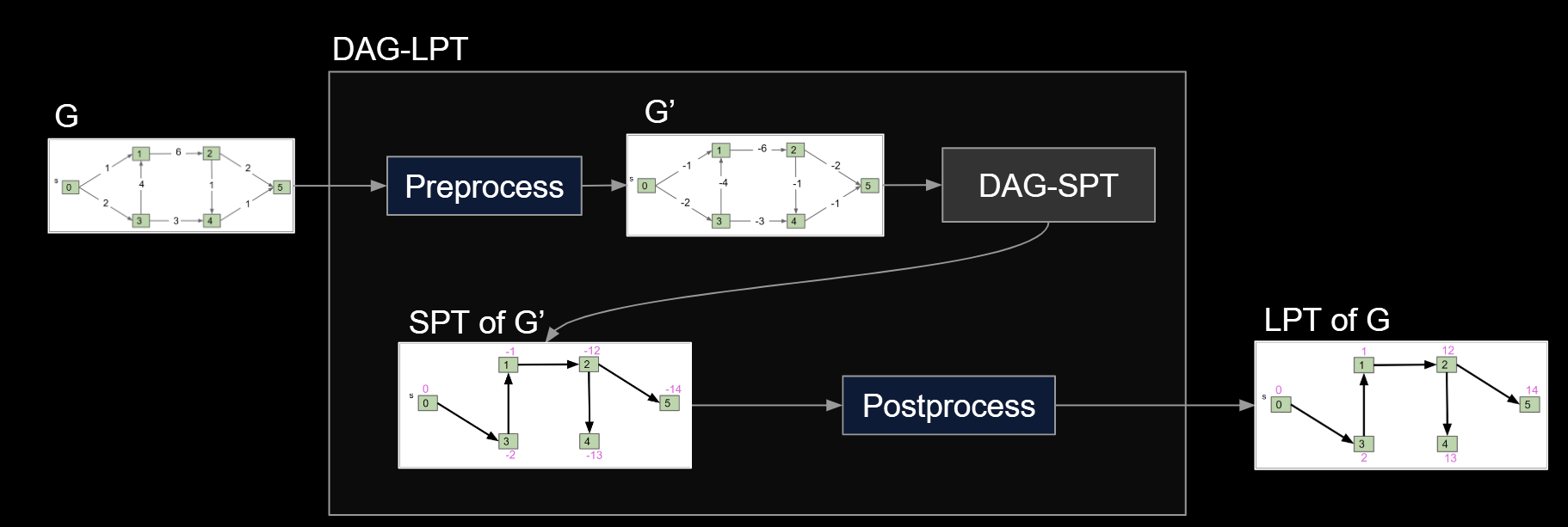
Question: Solve the LPT problem on a directed acyclic graph. Algorithm must be O(E + V) runtime.
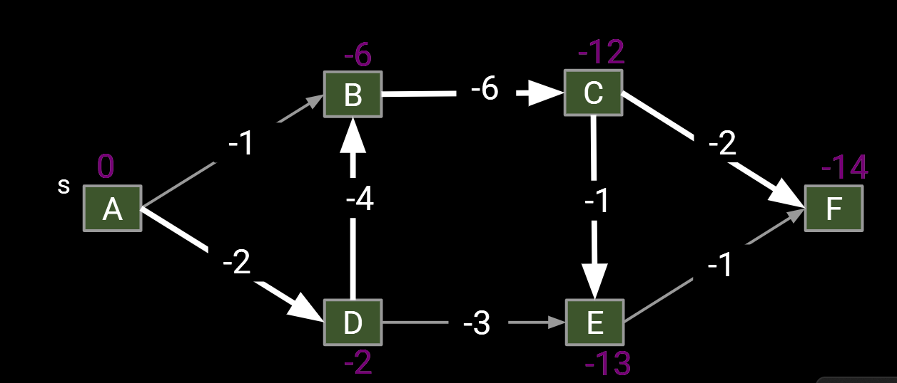
- Form a new copy of the graph G’ with signs of all edge weights flipped.
- Run DAGSPT on G’ yielding result X.
- Flip signs of all values in X.distTo. X.edgeTo is already correct.
14.4.Reductions: Definition
The problem solving we just used probably felt a little different than usual:
-
Given a graph G, we created a new graph G’ and fed it to a related (but different) algorithm, and then interpreted the result.
-
Since DAG-SPT can be used to solve DAG-LPT, we say that “DAG-LPT reduces to DAG-SPT”.
“If any subroutine for task Q can be used to solve P, we say P reduces to Q.”
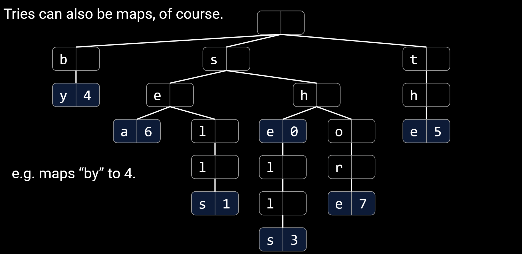
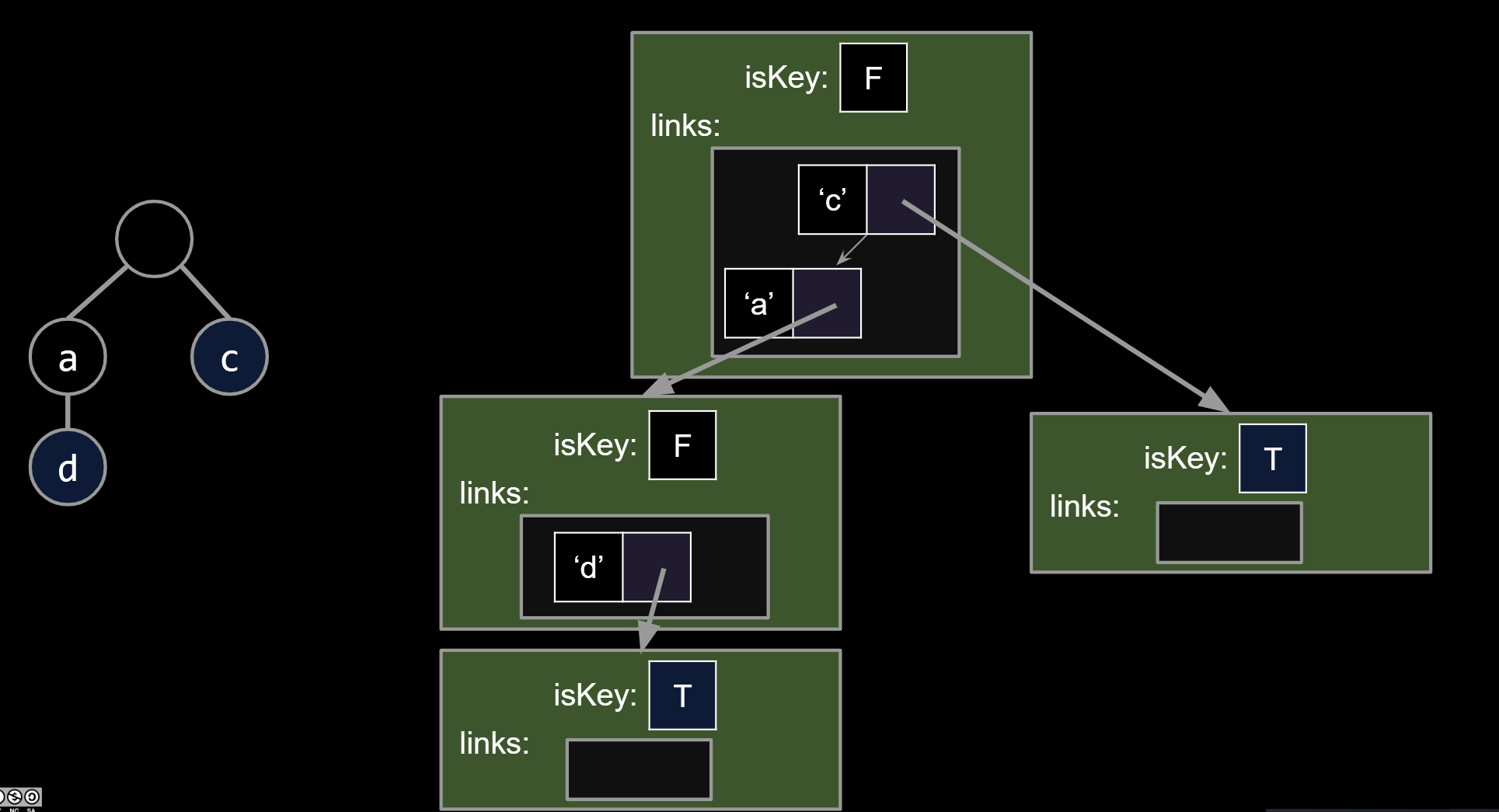
15.Tries
For String keys, we can use a “Trie”. Key ideas:
- Every node stores only one letter.
- Nodes can be shared by multiple keys.
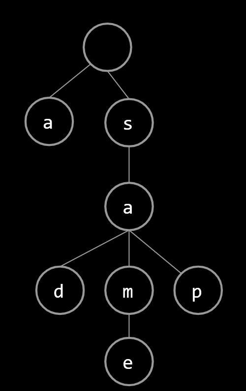
Above, we show the results of adding “sam”,“a”, “sap”, “same” and sad”.
Two ways to have a search “miss”:
- If the final node is white.
- If we fall off the tree, e.g. contains(“sax”).
15.1.Trie Implementation and Performance
The first approach might look something like the code below.
- Each node stores a letter, a map from c to all child nodes, and a color.
|
|
Each DataIndexedCharMap is an array of 128 possible links, mostly null.
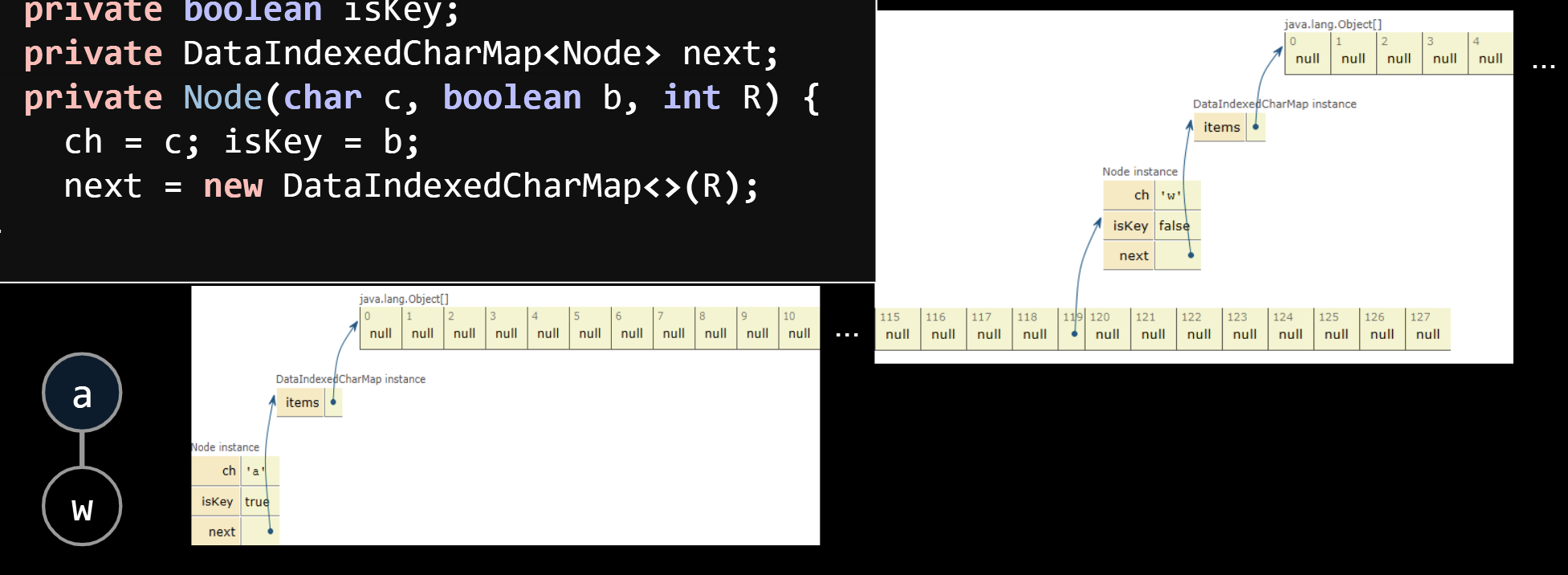
If we use a DataIndexedCharMap to track children, every node has R links.
Observation: The letter stored inside each node is actually redundant.
- Can remove from the representation and things will work fine.
|
|
| key type | get(x) | add(x) | |
|---|---|---|---|
| Balanced BST | comparable | Θ(log N) | Θ(log N) |
| Resizing Separate Chaining Hash Table | hashable | Θ(1)assuming even spread | Θ(1)on average,assuming even spread |
| data indexed array | chars | Θ(1) | Θ(1) |
| Tries | Strings | Θ(1) | Θ(1) |
One downside of the DataIndexedCharMap-based Trie is the huge memory cost of storing R links per node.
- Wasteful because most links are unused in real world usage.
15.2.Alternate Child Tracking Strategies
Using a DataIndexedCharMap is very memory hungry.
- Every node has to store R links, most of which are null.
Can use ANY kind of map from character to node, e.g.
-
BST
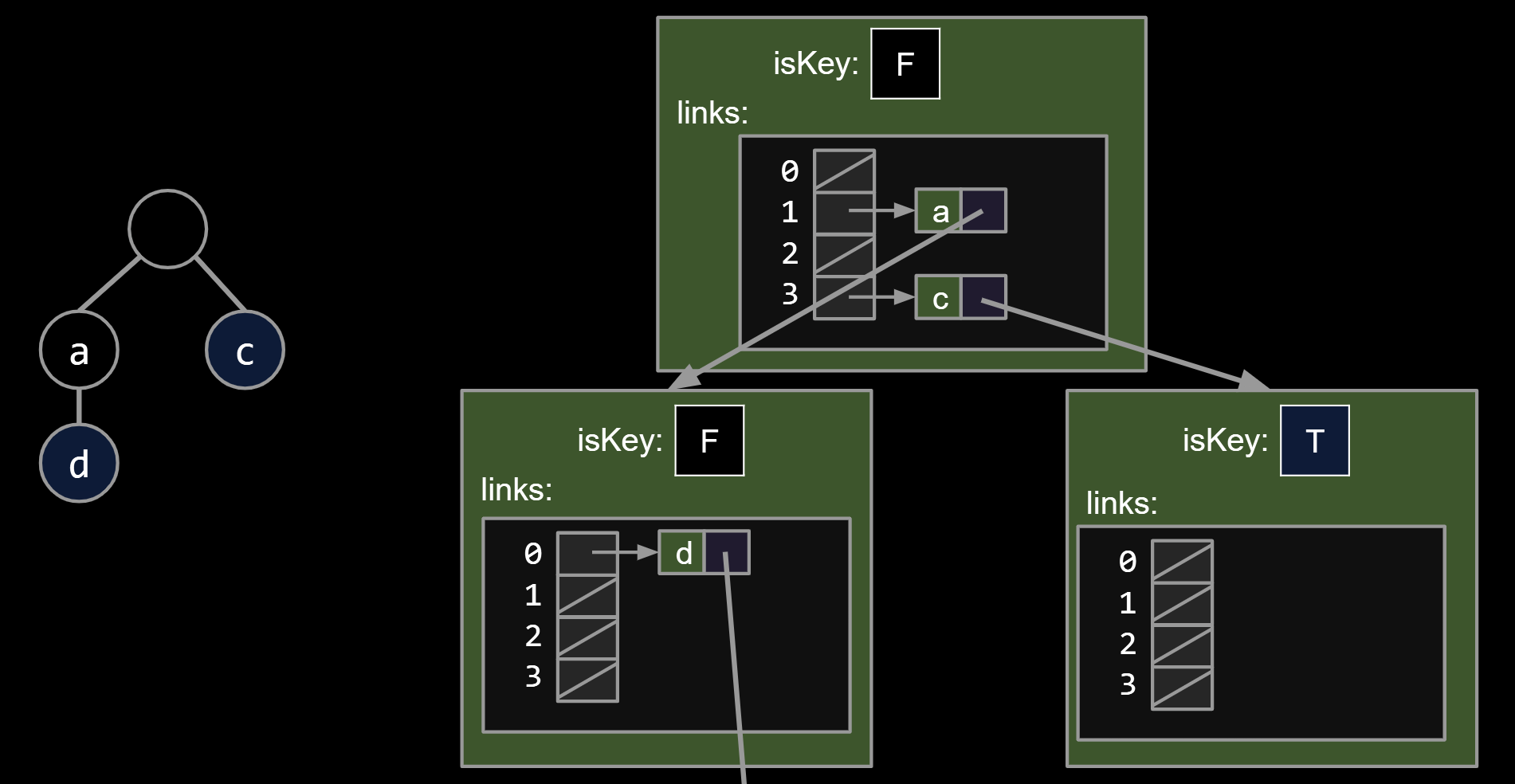
-
Hash Table
When our keys are strings, Tries give us slightly better performance on contains and add.
- Using BST or Hash Table will be slightly slower, but more memory efficient.
- Would have to do computational experiments to see which is best for your application.
- But where Tries really shine is their efficiency with special string operations!
15.3.Trie String Operations
Theoretical asymptotic speed improvement is nice. But the main appeal of tries is their ability to efficiently support string specific operations like prefix matching.
- Finding all keys that match a given prefix: keysWithPrefix(“sa”)
- Finding longest prefix of: longestPrefixOf(“sample”)
15.4.Autocomplete
Example, when I type “how are” into Google, I get 10 results.
One way to do this is to create a Trie based map from strings to values
- Value represents how important Google thinks that string is.
- Can store billions of strings efficiently since they share nodes.
- When a user types in a string “hello”, we:
- Call keysWithPrefix(“hello”).
- Return the 10 strings with the highest value.
16.Basic Sorts
16.1.Selection Sort
The logic:
- Start from the first element.
- Find smallest item after it.
- Swap this item to the front and ‘fix’ it.
- Repeat for unfixed items until all items are fixed.
Sort Properties:
- $Θ(N^2)$ time if we use an array (or similar data structure).
16.2.Inplace Heapsort
Idea: Instead of rescanning entire array looking for minimum, maintain a heap so that getting the minimum is fast!
For reasons that will become clear soon, we’ll use a max-oriented heap.
Naive heapsorting N items:
- Insert all items into a max heap, and discard input array. Create output array.
- Repeat N times:
- Delete largest item from the max heap.
- Put largest item at the end of the unused part of the output array.
Heap sorting N items:
- Use a process known as “bottom-up heapification” to convert the array into a heap.
- Repeat N times:
- Delete largest item from front of the heap.
- Put largest item at the end of the unused part of the array.
| Best Case Runtime | Worst Case Runtime | Space | Demo | Notes | |
|---|---|---|---|---|---|
| Selection Sort | $Θ(N^2)$ | $Θ(N^2)$ | $Θ(1)$ | Link | |
| Heapsort (in place) | $Θ(N)$ | $Θ(N \log N)$ | $Θ(1)$ | Link | Bad cache (61C) performance. |
17.Mergesort, Insertion Sort, and Quicksort
Merging can give us an improvement over vanilla selection sort:
- Selection sort the left half: Θ(N2).
- Selection sort the right half: Θ(N2).
- Merge the results: Θ(N).
Runtime is still Θ(N2), but faster since N+2*(N/2)2 < N2
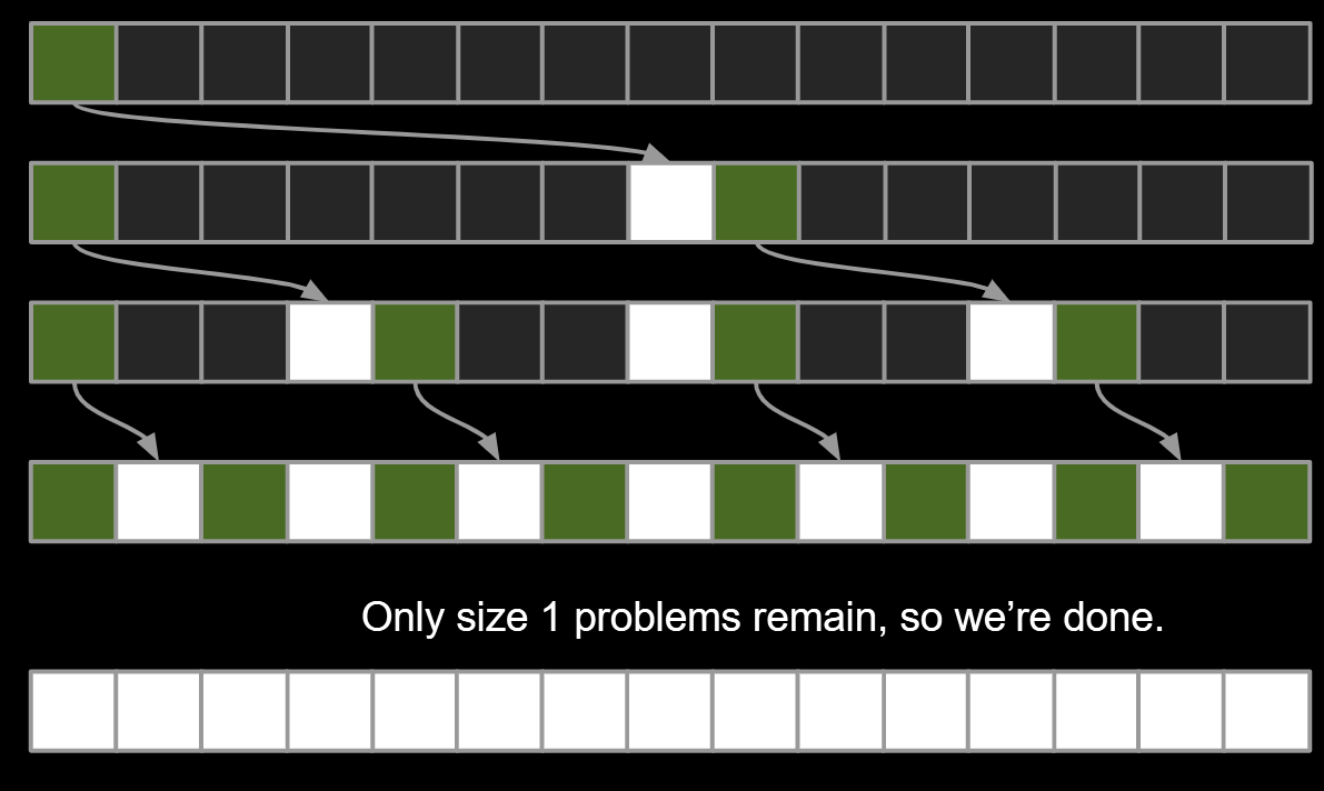
Mergesort has worst case runtime = Θ(N log N).
- Every level takes ~N AU.
- Top level takes ~N AU.
- Next level takes ~N/2 + ~N/2 = ~N.
- One more level down: ~N/4 + ~N/4 + ~N/4 + ~N/4 = ~N.
- Thus, total runtime is ~Nk, where k is the number of levels.
- How many levels? Goes until we get to size 1.
- k = log2(N).
- Overall runtime is Θ(N log N).
Mergesort:
- Split items into 2 roughly even pieces.
- Mergesort each half (steps not shown, this is a recursive algorithm!)
- Merge the two sorted halves to form the final result.
- Also possible to do in-place merge sort, but algorithm is very complicated, and runtime performance suffers by a significant constant factor.
| Best Case Runtime | Worst Case Runtime | Space | Demo | Notes | |
|---|---|---|---|---|---|
| Selection Sort | Θ(N2) | Θ(N2) | Θ(1) | Link | |
| Heapsort (in place) | Θ(N)* | Θ(N log N) | Θ(1)** | Link | Bad cache (61C) performance. |
| Mergesort | Θ(N log N) | Θ(N log N) | Θ(N) | Link | Faster than heap sort. |
17.1.Naive Insertion Sort and In-Place Insertion Sort
Naive Insertion Sort
General strategy:
- Starting with an empty output sequence.
- Add each item from input, inserting into output at right point.
In-Place Insertion Sort
- General strategy:
- Repeat for i = 0 to N - 1:
- Designate item i as the traveling item.
- Swap item backwards until traveler is in the right place among all previously examined items.
- Repeat for i = 0 to N - 1:
| Best Case Runtime | Worst Case Runtime | Space | Demo | Notes | |
|---|---|---|---|---|---|
| Selection Sort | Θ(N2) | Θ(N2) | Θ(1) | Link | |
| Heapsort (in place) | Θ(N)* | Θ(N log N) | Θ(1) | Link | Bad cache (61C) performance. |
| Mergesort | Θ(N log N) | Θ(N log N) | Θ(N) | Link | Fastest of these. |
| Insertion Sort (in place) | Θ(N) | Θ(N2) | Θ(1) | Link | Best for small N or almost sorted. |
18. Partition Sort, a.k.a. Quicksort
To partition an array a[] on element x=a[i] is to rearrange a[] so that:
- x moves to position j (may be the same as i)
- All entries to the left of x are <= x.
All entries to the right of x are >= x
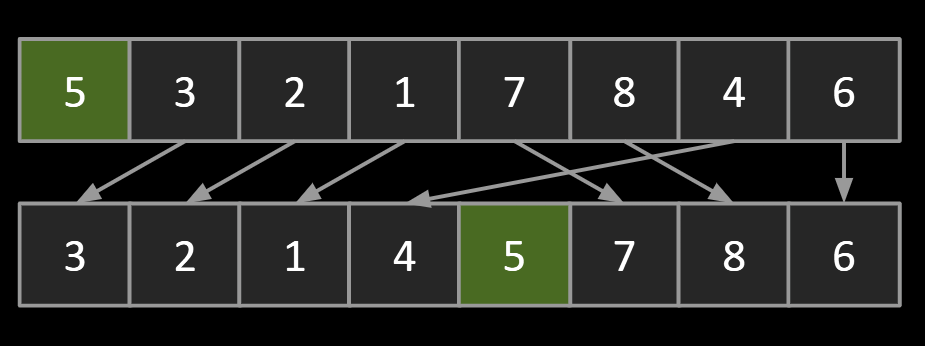
Observations:
- 5 is “in its place.” Exactly where it’d be if the array were sorted.
- Can sort two halves separately, e.g. through recursive use of partitioning.
Quick sorting N items:
- Partition on leftmost item.
- Quicksort left half.
- Quicksort right half.
18.1.Runtime
Theoretical analysis:
- Partitioning costs Θ(K) time, where Θ(K) is the number of elements being partitioned (as we saw in our earlier “interview question”).
- The interesting twist: Overall runtime will depend crucially on where pivot ends up.
- Best Case: Pivot Always Lands in the Middle
Overall runtime:
Θ(NH) where H = Θ(log N)
so: Θ(N log N)
- Worst Case: Pivot Always Lands at Beginning of Array
What is the runtime Θ(∙)?
- $N^2$
- but overall, the runtime is roughly $\Theta(\log N)$
18.2.Avoiding Quicksort Worst Case
What can we do to avoid worst case behavior? Four philosophies:
- Randomness: Pick a random pivot or shuffle before sorting.
- Smarter pivot selection: Calculate or approximate the median.
- Introspection: Switch to a safer sort if recursion goes to deep.
- Try to cheat: If the array is already sorted, don’t sort (this doesn’t work).
Implement: Create L and G pointers at left and right ends.
- L pointer is a friend to small items, and hates large or equal items.
- G pointer is a friend to large items, and hates small or equal items.
- Walk pointers towards each other, stopping on a hated item.
- When both pointers have stopped, swap and move pointers by one.
- When pointers cross, you are done. See This site
19. Software Engineering
There are two kinds of complexity:
- Unavoidable (Essential) Complexity
- Inherent, inescapable complexity caused by the underlying functionality
- Avoidable Complexity
- Complexity that we can address with our choices
In response to avoidable complexity, we can:
- Make code simpler and more obvious
- Using sentinel nodes in Project 1
- Modules
- Abstraction: the ability to use a piece without understanding how it works based on some specification
- Interfaces - HashMap, BSTMap both are Maps
19.1. Strategic vs Tactical Programming
A different form of programming that emphasizes long term strategy over quick fixes. The objective is to write code that works elegantly - at the cost of planning time.
Code should be:
- Maintainable
- Simple
- Future-proof
If the strategy is insufficient, go back to the drawing board before continuing work.
19.2. Design
Design is an important first stage in development:
- Ensures consideration of all requirements and constraints
- Considers multiple alternatives and their advantages / disadvantages
- Identifies potential costs or pitfalls while change is cheap
- Allows multiple minds to weigh in and leverages diverse perspectives
Design documents do not need to follow a specific form, but they should give the reader easily accessible information about your project.
A design document should:
- Quickly bring the reader up to speed
- Include what alternatives were considered and why the trade-offs were made
- Be just as much about the “why” as it is about the “how”
- Update as the project progresses (be alive!)
- Look up THIS SITE
19.3. Managing Complexity
What is “good code”? Three main goals:
- Readability: The code is easy to read and understand.
- Simplicity: The solution is straightforward, without unnecessary complexity
- Testability: The code is easy to test and debug.
19.4. Documentation
- Documentation in technology refers to various written materials that accompany software or systems
- It covers a broad spectrum, including:
- Code Comments
- API Documentation
- User Manuals
- Design Specifications
- Test Documents
|
|